Diatom based transfer function for estimating the chemical composition of fossil water. Calibration based on salt lakes of the Lipez area in the southwestern Bolivian Altiplano

Servant-Vildary, Simone ; Risacher, François; Roux, Maurice; Risacher, François; Roux, Maurice

F. ILLUSTRATIONS

Figures

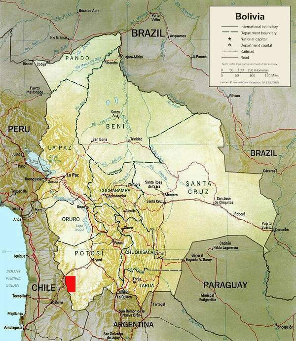
Figure 1: Map of Bolivia. Map showing the location of the western Lipez. From West to East, the area is divided into 4 main geomorphic units: the Western Cordillera, the Altiplano, the Eastern Cordillera and the Amazonian "llanos".
Figure 2: Location of the lakes. Location of the lakes where modern diatoms have been studied in the Pastos Grandes area. See Figure 4 for the locations of Laguna Colorada, Puripica and Laguna Verde lakes, sited farther south (after Ballivián & Risacher, 1981, modified).
Figure 3: Pastos Grandes. Location of the surface sediment samples taken for diatom analyses.
Figure 4: Location of the lakes. Location of the lakes in the Lipez area where water chemistry was studied.
Figure 5A: WA method. Estimated optima and tolerances of 61 species to salinity (All with maximum abundance > 3 and occurrence in three or more samples).
Figures 5B and 5C: WA method. Estimated optima and tolerances of 61 species to alkalinity (with maximum abundance > 3 and occurrence in three or more samples). In Figure 5C, the very high values of alkalinity were removed in order to show more clearly the optima and tolerances of species with low alkalinity values

Figures 6A and 6B: WA-PLS method. The salinity and alkalinity of the lakes as inferred from modern diatom assemblages (calibration).

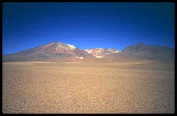
Figure 7: An example of the Lipez landscape: In the foreground a Quaternary glacis with a pebble cover. Note the absence of vegetation. In the background an Upper Cenozoic volcano.
Figure 8: Laguna Chiar Kkota in the foreground and Laguna Hedionda in the background. Salt deposits fringe the lakes.
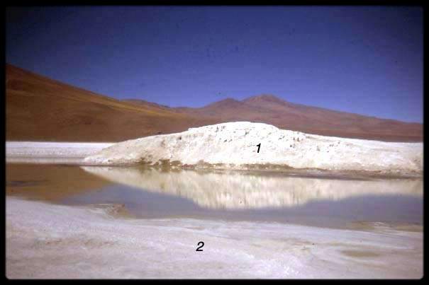
Figure 9: Laguna Ballivián: Playa-type "salar", characterized by a very small watershed.
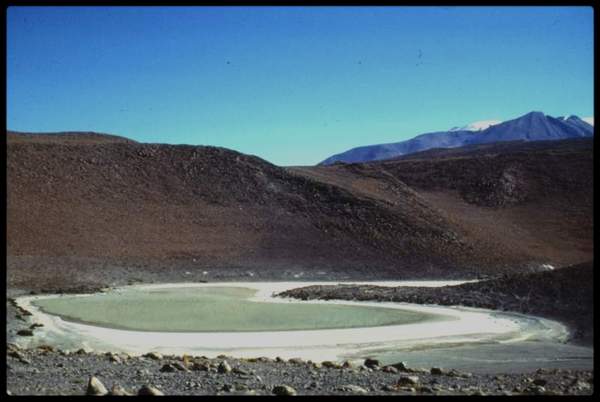
Figure 10: Laguna Ramaditas: In the background the threshold which separates Laguna Ramaditas from Laguna Ballivián. The two lakes were connected during the "Minchin" highstand phase.
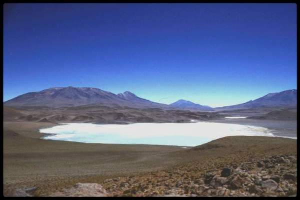
Figure 11: Laguna Honda. 1: Past shorelines with bioherms, the top one is dated early Holocene (~ 11.800 cal yr BP) by U/Th, 2: Undated lacustrine deposits, 3: Diatomites representing the three main lacustrine phases (Minchin, Tauca and Coipasa).
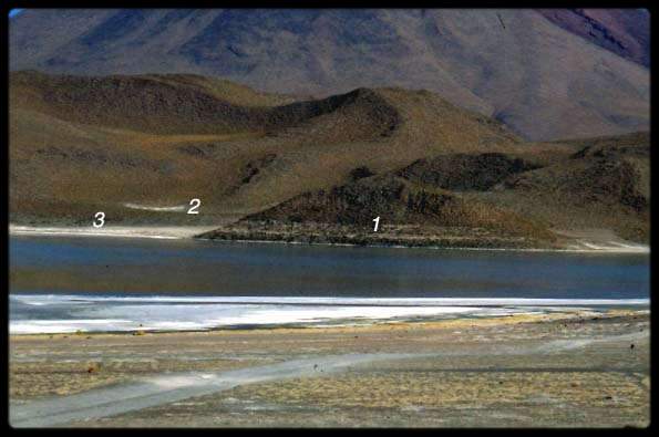
Figure 12: Cachi Laguna salar: Unconfined aquifer salar.
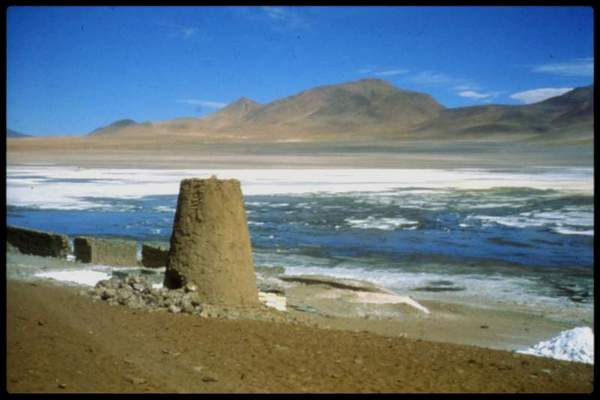
Figure 13: Laguna Colorada: 1: Springs at the foot of the slope, 2: Quaternary diatomites, 3: Open surface salt water.
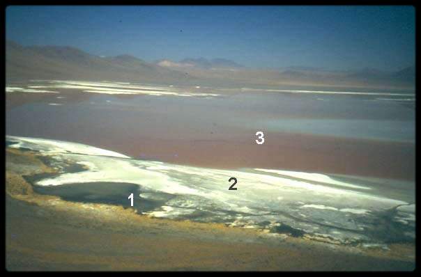
Figure 14: Pastos Grandes salar: Fossil calcareous crust (undated).
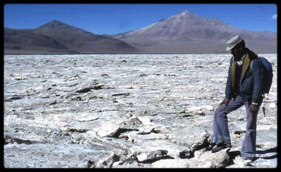
Figure 15: Pastos Grandes salar: Calcareous pisoliths in shallow ephemeral pools fed by hot springs. Diatomites are common in the outer layers.
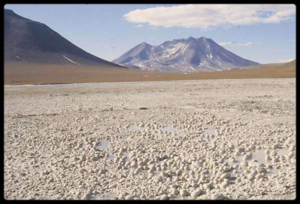
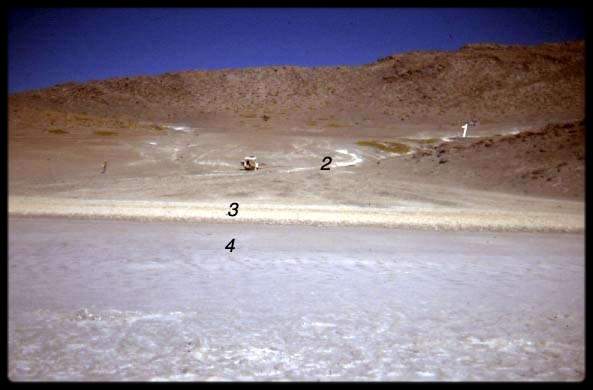
Figure 16: Laguna Ballivián: 1: Diatomites and bioherms of the highest water level, probably of the Minchin phase (Middle Glacial), 2: Diatomites presumably of the Tauca phase. Formations 1 and 2 are separated by an erosion surface, 3: Modern colluvions, 4: Halite efflorescences.
Figure 17: Laguna Ramaditas: Northern border. 1: Quaternary diatomites eroded by the wind during a Holocene dry phase, 2: Present-day halite efflorescences.

Tables

Table 1 : Location of the lakes and data regarding water chemistry.

Table 2 : List of species and their abundance in 30 samples.

Table 3 : List of diatom pictures.

Table 4 : WA method: Optima and tolerances of the species (in alphabetical order) to Na⁺, Mg⁺⁺, SO4^--, Si, Li⁺, salinity, pH, K⁺, Ca⁺⁺, Cl^-, B and alkalinity. Estimation of environmental variables for each sample. SEP values are indicated at the end of the list of estimations for all samples. Optima and tolerances of species to salinity and alkalinity are illustrated in Figures 5A , 5B and 5C .
WA-PLS method. Values of r, R, R² and SEP listed in table 4 show that this method improves the predictions for all the environmental parameters. Calibration of salinity and alkalinity is illustrated in Figures 6A and 6B .