◄ Carnets Geol. 16 (1) ►
![]()
Contents
[Introduction]
[... the Unitary Associations method]
[... 's data on the Paleogene]
[Results of the computation] [Discussion]
[The transgressive-regressive patterns ...]
[Conclusions] [Bibliographic references]
and ... [Appendices]
(Sortable tables: [Table 1]
[Table 2]
[Appendix 1]
[Appendix 2.1]
[Appendix 2.2]
[Appendix 2.3]
[Appendix 2.4] and
[Appendix 2.5])
Institute of Earth Sciences, University of Lausanne,
G�opolis, CH-1015 Lausanne (Switzerland)
Department of Geological Sciences, Jackson School of Geosciences, University of Texas at Austin, 2275 Speedway Stop C9000, Austin, TX 78712 � 1722 (USA)
Published online in final form (pdf) on January 14, 2016
[Editor: Bruno ;
language editor: Don ]
![]()
The relative diachronism of first or last local occurrences (FOs and LOs) of fossil species may highlight transgressive/regressive cycles. A simple technique allowing the extraction of this information by means of the UAgraph program is discussed in the present paper. The technique consists in modifying a usual database of UAgraph by augmenting it with the restricted data concerning only the FOs (or LOs) of the taxa under consideration. The resulting data set combines the information on total ranges and those concerning the FOs and LOs only. Calculating the UAs of such a duplicated database produce a range chart in which we can read the maximal ranges of all the taxa and, in addition, the biochronological dispersion of the FOs and LOs. For a given transgressive/regressive cycle, the UAs defined by the species related to sea level fluctuations migrate with time from distal to proximal sections and inversely. This trend can be detected visually by the means of the UAs reproducibility chart, output of the UAgraph program. In a more general frame, the same holds true for species whose regional dispersion is related to specific conditions and when these conditions migrate in space with time (e.g., water temperatures and diatoms). The above discussion is strictly related to FOs and LOs that for a given section are definitive, however well constrained ephemeral appearances and disappearances can be easily integrated in the database for the same purposes.
Diachronism of datums; transgressive/regressive cycles; ; UAgraph program.
J. & F. (2016).- A simple technique to establish sequences of datums and to highlight transgressive�regressive cycles.- Carnets Geol., Madrid, vol. 16, nº 1, p. 1-16.
Une technique simple pour identifier des s�quences de points de r�f�rence et mettre en �vidence des cycles transgressifs et r�gressifs.- Le diachronisme des premi�res et derni�res occurrences (FOs et LOs) des esp�ces fossiles permettent dans certains cas de mettre en �vidence des cycles transgressifs et r�gressifs. Nous d�crivons ici une technique simple pour extraire ces informations avec l'aide du programme UAgraph. Cette technique consiste � d�doubler la base usuelle de donn�es stratigraphiques en consid�rant simultan�ment les extensions stratigraphiques totales des esp�ces en y ajoutant l'information sur leurs premi�res occurrences locales. Si l'on calcule les associations unitaires d'une telle base de donn�es, on obtient simultan�ment une vision claire des dur�es d'existences globales des esp�ces et le diachronisme des FOs (ou LOs) qui leur sont associ�es. Ces r�sultats compl�mentaires permettent d'affiner la recherche de cycles s�dimentaires dans les donn�es initiales en augmentant le pouvoir de r�solution du programme UAgraph.
Diachronisme de points de r�f�rences ; cycles transgressifs-regressifs ; ; programme UAgraph.
This paper is dedicated to the memory of Rosemary who passed away much too young after a brilliant start to her scientific career. Her work on the stratigraphic data of Antarctic diatoms gave rise to a very challenging paper ( et al., 2008) that, among other, served as basis for several in depth analyses of the well known Conop program ( et al., 2010; et al., 2015).
Palaeontologists are well aware that the first and last local occurrences (FOs and LOs) of fossil species are never really synchronous in locations that are remote from each other. If a datum is found in different biostratigraphic zones in different locations, we say it is diachronous and the datums' biochronological dispersion is equal to the number of units separating the oldest occurrence of the FO of a given taxon in a given locality and the highest FO of the same taxon in some other locality (, 1979).
The most usual case of inter-datum diachronism is illustrated in
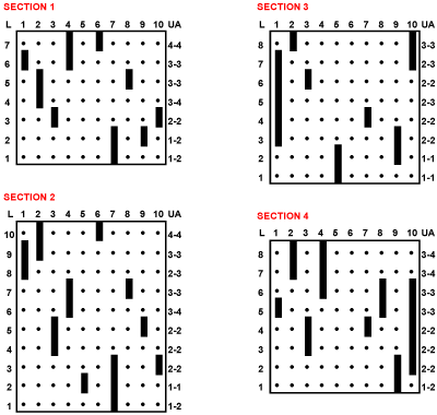
Fig. 1 ![]() showing that the relative stratigraphic positions observed locally among fossil species commonly are not constant from one place to the other: most species occupy apparently contradictory positions in the four different locations of our diagram.
showing that the relative stratigraphic positions observed locally among fossil species commonly are not constant from one place to the other: most species occupy apparently contradictory positions in the four different locations of our diagram.
 |
 |
|
| A | B |
Click on thumbnail to enlarge the image.
Figure 1: Local stratigraphic distribution of 10 species (1�10). The relative positions of the first local appearances of the 10 species in these sections are diachronous from one section to the other and are represented in Fig. 1.B. UA 1 to 4 are units of a discrete time scale calculated using the "Unitary Associations method" (, 1991, see below).
That diagram is based on the local stratigraphic distributions of the 10 taxa represented in
Fig. 1.A ![]() and shows that the lines of correlations linking the first occurrences of the taxa in the 4 different localities are affected by a multitude of crossovers, making it difficult to distinguish a chronologically significant event allowing a reliable correlation of the different stratigraphic sections. That diagram also illustrates the fact that the stratigraphic position of a given taxon x can be recorded anywhere within its total existence interval, leading to contradictive chronological positions in the different fossil localities where the taxon is found.
and shows that the lines of correlations linking the first occurrences of the taxa in the 4 different localities are affected by a multitude of crossovers, making it difficult to distinguish a chronologically significant event allowing a reliable correlation of the different stratigraphic sections. That diagram also illustrates the fact that the stratigraphic position of a given taxon x can be recorded anywhere within its total existence interval, leading to contradictive chronological positions in the different fossil localities where the taxon is found.
Suppose that we have only paleontological data to demonstrate which of two contradictive datums is older than the other one, in the absence of any physical proxy (paleomagnetism, geochronology, lithological marker bed, etc.). The only way to solve such a problem is to consider the stratigraphic position of the contradictive datums in relation to the taxa that are characteristic of the units of a discrete time scale (i.e., the zones = defined as an order relation). This allows to demonstrate that one datum is older in a given section than in another. For
example, in
Fig. 1 ![]() ,
taxon 1 first occurs in zone UA3 in sections 1, 2 and 4 and in UA2 in section 3.
,
taxon 1 first occurs in zone UA3 in sections 1, 2 and 4 and in UA2 in section 3.
A fundamental theorem of graph theory is hidden behind the above statement. It is indeed important to keep in mind that the uniqueness of a coexistence interval of n species (a clique) can be established based on fragmentary biostratigraphic data coming from many localities (at most (n2 - n)/2 localities in which only a pair of species is found each time). This fundamental property of cliques whose vertices (i.e., the points of the graph) represent intervals is called 's theorem (proof in , 1987) and it can be stated as follows:
"If a family of intervals does not contain two disjoint intervals, then a point exists that is common to all of them."
That theorem can easily be proven as follows. At least one interval of the family has a maximal lower bound and at least one interval of the family has a minimal upper bound. By hypothesis, those two intervals intersect and their intersection is that of the family.
From this theorem we can propose a formal graph theoretical definition of the diachronism. If the FO (or LO) of a given taxon is located below a maximal intersection in a given locality and above it in another locality, it is diachronous.
The Unitary Associations method is designed for the construction of concurrent range zones using a fully deterministic approach. The basic idea is to construct a discrete sequence of coexistence intervals of species. Each interval, corresponding to one UA, consists of a maximal set of intersecting ranges (i.e., not included in a larger set). Each UA is characterized by a set of species (or exclusive pairs of species) allowing its recognition in the stratigraphic sections. A given UA is distinguished from the previous UA by at least the disappearance of an older species and the appearance of a new species.
The sole disappearance of an old species results in the younger set of species to be included in the older one; and the sole appearance of a new species results in the older set of species to be included in the younger one. The understanding of this trivial fact is fundamental for the understanding of the technique discussed in this paper. The basic steps of the method are as follows. The data are compiled into a presence�absence matrix, with samples in rows and taxa in columns. From these data, maximal sets of mutually co-occurring species (maximal cliques) are constructed. Stratigraphical superpositions of maximal cliques are then inferred from the observed superpositional relationships between the taxa they contain. The longest possible sequence of superposed maximal cliques is then used to construct a sequence of UAs. Finally, the original samples are assigned to UAs whenever possible and are thus stratigraphically correlated. A full description of the Unitary Associations method and of the UAgraph computer program can be found in et al. (2015).
The following discussion concerns transgressive/regressive cycle characterised by UAs defined by FOs and LOs related to sea level fluctuations. However in a more general frame, it could be applied to all datasets containing species whose spatial distribution is related to specific conditions that vary with time (e.g., sea water temperatures and diatoms).
During transgressive/regressive cycles the occurrences of species sensible to bathymetric fluctuations (e.g., benthic foraminifera) migrate with time from distal to proximal sections and inversely. We will show below that such trends can be detected visually by means of the UAs reproducibility chart, output of the UAgraph program ( et al., 2015).
As a real example we will use again the beautiful data of and
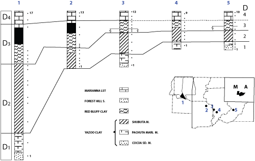
(1963) and (1965) on the Paleogene benthic foraminifera and ostracods from Mississipi and Alabama in five sections located along a "deep water to shallow water" transect
(Fig.
2 ![]() ). collected 155 different taxa in his sections and the code numbers of these taxa are given in
Appendices 1 and 2. (loc. cit.) began his comprehensive biostratigraphic study of the Paleogene west of Alabama and east of Mississippi. His goal was two-fold: first, to solve some problems posed by correlating the lithologic units classically used in this region
(Fig. 1
). collected 155 different taxa in his sections and the code numbers of these taxa are given in
Appendices 1 and 2. (loc. cit.) began his comprehensive biostratigraphic study of the Paleogene west of Alabama and east of Mississippi. His goal was two-fold: first, to solve some problems posed by correlating the lithologic units classically used in this region
(Fig. 1 ![]() ) and second, to use new biochronologic arguments to determine more precisely the boundary between the Jacksonian and Vicksburgian stages. His investigations concerned mainly the distribution of foraminifera and ostracods in his five sections which were sampled in great detail.
) and second, to use new biochronologic arguments to determine more precisely the boundary between the Jacksonian and Vicksburgian stages. His investigations concerned mainly the distribution of foraminifera and ostracods in his five sections which were sampled in great detail.
Since then, his remarkable results have been used by (1970, 1977), (1970), et al. (1978), (1985), (1991) and et al. (2015) in an attempt to establish quantitative correlations with the help of a number of statistical methods (cluster analysis, RBV, lateral tracing, etc.).
The unitary associations can be applied to such a problem in different ways.
1) The easiest method, as has been already demonstrated by (1991) and et al. (2015), consists in recognizing the differential distribution of the biostratigraphic zones defined by UAs in proximal versus distal sections. Regressive cycles are marked by the absence, in proximal sections, of biostratigraphic zones which are observed in distal sections. High stands of the sea level are recognized by the ubiquitous distribution of a biostratigraphic zone. This approach applied to the 's problem results in the identification of two regressive phases located at the basis of the Shubuta Member and the base of the Red Bluff Clay Member.
2) A different approach consists in establishing a biostratigraphic zonation where zones represent well-constrained discrete units with a strong superpositional control and an accurate lateral traceability, i.e., zone of unitary associations (UA-zones). The distribution of these zones in the sedimentary basin can be seen as non-intersecting lines of correlation. A line that ties the local occurrences of a given datum is diachronous when it intersects one or more UAs zones. In the case of a species particularly sensible to bathymetric conditions, the progressive intersection between its FOs and younger UA zones from distal to proximal sections could be indicative of a transgressive phase. The reproducibility of this observation for a great number of species and the same set of UAs zone allows the recognition of a transgressive phase. This method is probably the most robust, but its application is time consuming.
3) The goal of the present paper is to provide an alternative method to establish a sequence of unitary associations by combining species total ranges of the taxa and their first occurrences. That new technique is applied below to the 's problem.
The usual way to compile biostratigraphic data from several stratigraphic sections consists in giving the stratigraphic range of each taxon xi expressed as the levels of its first and last local occurrence (FO and LO) in that section. For example if taxon x1 is found in section A where 10 levels are studied, we start by writing "Section A, bottom 1 top 10". Then we write x1,3,7 if x1 first occurs in level 3 and disappears locally in level 7. It is clearly impossible to have a simpler input than this one. In the UAgraph program terminology, such an input is said to have the format "DATUM" (= triples of codes).
The technique used here to highlight transgressive/regressive cycles by the means of UAgraph consists in enlarging this usual database by augmenting it with the restricted data concerning only the FOs (or LOs) of the taxa under consideration in each section. For example, if we take the local range of taxon x1 in section A mentioned above, we will obtain the following augmented stratigraphic information x1,3,7 followed by FOx1,3,3 (i.e., the first local occurrence of taxon x1 is observed in level 3). Doing so for all the stratigraphic data in a given database, we obtain a duplicated data set combining the information on total ranges and those concerning the FOs only (or LOs only, that we will ignore in the present discussion for reasons of simplicity).
's original sections are reproduced in Fig.
2 ![]() and the database extracted from his paleontological study is given in
Appendix 2. Table 1 shows how the augmented database appears when completed by the data concerning the FOs. When calculating unitary association from such a kind of augmented database, first and last occurrences of species are treated as events which are not instantaneous, a philosophy that in most cases matches the observed biostratigraphic record. Therefore, a given FO (or LO) can have a range in the resulting range chart, exactly like an usual fossil species. The length of the range corresponds to the biochronological dispersion of the event within the considered database.
and the database extracted from his paleontological study is given in
Appendix 2. Table 1 shows how the augmented database appears when completed by the data concerning the FOs. When calculating unitary association from such a kind of augmented database, first and last occurrences of species are treated as events which are not instantaneous, a philosophy that in most cases matches the observed biostratigraphic record. Therefore, a given FO (or LO) can have a range in the resulting range chart, exactly like an usual fossil species. The length of the range corresponds to the biochronological dispersion of the event within the considered database.
Click on thumbnail to enlarge the image.
Figure 2: 's sections 1 to 5: 1 Wayne and Clark Counties (composite section), 2 St Stephen Quarry, 3 Little Stave Creek, 4 Jackson, 5 Perdue Hill.
Table 1: Part of the duplicated 's database showing the 50 first taxa of the first section from the total database given in the Appendix 2. Left columns: total local ranges. Second columns: FO only.
| x | FO | LO | FOx | FO | FO | |
| 1 | 12 | 15 | FO 1 | 12 | 12 | |
| 2 | 11 | 15 | FO 2 | 11 | 11 | |
| 3 | 4 | 8 | FO 3 | 4 | 4 | |
| 5 | 7 | 8 | FO 5 | 7 | 7 | |
| 6 | 4 | 8 | FO 6 | 4 | 4 | |
| 7 | 3 | 8 | FO 7 | 3 | 3 | |
| 8 | 4 | 6 | FO 8 | 4 | 4 | |
| 9 | 4 | 11 | FO 9 | 4 | 4 | |
| 10 | 4 | 8 | FO10 | 4 | 4 | |
| 11 | 4 | 8 | FO13 | 4 | 4 | |
| 14 | 1 | 10 | FO14 | 1 | 1 | |
| 15 | 3 | 10 | FO15 | 3 | 3 | |
| 16 | 1 | 8 | FO16 | 1 | 1 | |
| 17 | 4 | 17 | FO17 | 4 | 4 | |
| 18 | 15 | 15 | FO18 | 15 | 15 | |
| 19 | 1 | 3 | FO19 | 1 | 1 | |
| 20 | 4 | 4 | FO20 | 4 | 4 | |
| 21 | 14 | 15 | FO21 | 14 | 14 | |
| 22 | 5 | 17 | FO22 | 5 | 5 | |
| 23 | 1 | 10 | FO23 | 1 | 1 | |
| 24 | 14 | 17 | FO24 | 14 | 14 | |
| 26 | 2 | 6 | FO26 | 2 | 2 | |
| 27 | 16 | 17 | FO27 | 16 | 16 | |
| 28 | 2 | 17 | FO28 | 2 | 2 | |
| 30 | 3 | 14 | FO30 | 3 | 3 | |
| 31 | 1 | 2 | FO31 | 1 | 1 | |
| 32 | 2 | 2 | FO32 | 2 | 2 | |
| 34 | 3 | 8 | FO34 | 3 | 3 | |
| 35 | 3 | 15 | FO35 | 3 | 3 | |
| 36 | 16 | 17 | FO36 | 16 | 16 | |
| 38 | 3 | 10 | FO38 | 3 | 3 | |
| 39 | 1 | 3 | FO39 | 1 | 1 | |
| 40 | 4 | 7 | FO40 | 4 | 4 | |
| 41 | 3 | 11 | FO41 | 3 | 3 | |
| 43 | 16 | 16 | FO43 | 16 | 16 | |
| 44 | 4 | 8 | FO44 | 4 | 4 | |
| 45 | 4 | 16 | FO45 | 4 | 4 | |
| 46 | 3 | 9 | FO46 | 3 | 3 | |
| 47 | 3 | 9 | FO47 | 3 | 3 | |
| 48 | 4 | 6 | FO48 | 4 | 4 | |
| 50 | 4 | 7 | FO50 | 4 | 4 |
To show the results of the above operation applied to the complete database, we give the numerical range chart of the total ranges of the taxa 1 to 155 together with the diachronism of their FO in the different sections (Table 2).
Table 2: Numerical range chart calculated by means of UAgraph showing the biochronological dispersion of the FO of taxa 1 to 155, denoted as FOx,a,b. The total ranges of the taxa are denoted as x,a,b.
| FOx | x | First UA | Last UA |
| FO 1 | 5 | 30 | |
| 1 | 5 | 39 | |
| FO 2 | 23 | 33 | |
| 2 | 23 | 39 | |
| FO 3 | 4 | 19 | |
| 3 | 4 | 33 | |
| FO 4 | 33 | 39 | |
| 4 | 33 | 39 | |
| FO 5 | 13 | 22 | |
| 5 | 13 | 23 | |
| FO 6 | 5 | 20 | |
| 6 | 5 | 26 | |
| FO 7 | 11 | 16 | |
| 7 | 11 | 22 | |
| FO 8 | 14 | 19 | |
| 8 | 14 | 26 | |
| FO 9 | 15 | 23 | |
| 9 | 15 | 33 | |
| FO 10 | 7 | 21 | |
| 10 | 7 | 26 | |
| FO 11 | 27 | 34 | |
| 11 | 27 | 39 | |
| FO 12 | 8 | 18 | |
| 12 | 8 | 33 | |
| FO 13 | 12 | 19 | |
| 13 | 12 | 28 | |
| FO 14 | 3 | 16 | |
| 14 | 3 | 26 | |
| FO 15 | 11 | 17 | |
| 15 | 11 | 26 | |
| FO 16 | 3 | 13 | |
| 16 | 3 | 33 | |
| FO 17 | 19 | 31 | |
| 17 | 19 | 40 | |
| FO 18 | 24 | 36 | |
| 18 | 24 | 39 | |
| FO 19 | 2 | 7 | |
| 19 | 2 | 20 | |
| FO 20 | 13 | 19 | |
| 20 | 13 | 23 | |
| FO 21 | 32 | 33 | |
| 21 | 32 | 39 | |
| FO 22 | 22 | 38 | |
| 22 | 22 | 40 | |
| FO 23 | 1 | 5 | |
| 23 | 1 | 29 | |
| FO 24 | 28 | 33 | |
| 24 | 28 | 40 | |
| FO 25 | 37 | 39 | |
| 25 | 37 | 40 | |
| FO 26 | 2 | 23 | |
| 26 | 2 | 39 | |
| FO 27 | 31 | 39 | |
| 27 | 31 | 40 | |
| FO 28 | 5 | 10 | |
| 28 | 5 | 40 | |
| FO 29 | 1 | 31 | |
| 29 | 1 | 35 | |
| FO 30 | 1 | 14 | |
| 30 | 1 | 39 | |
| FO 31 | 3 | 31 | |
| 31 | 3 | 40 | |
| FO 32 | 10 | 16 | |
| 32 | 10 | 39 | |
| FO 33 | 12 | 31 | |
| 33 | 12 | 40 | |
| FO 34 | 11 | 16 | |
| 34 | 11 | 22 | |
| FO 35 | 11 | 14 | |
| 35 | 11 | 36 | |
| FO 36 | 13 | 38 | |
| 36 | 13 | 40 | |
| FO 37 | 5 | 16 | |
| 37 | 5 | 24 | |
| FO 38 | 5 | 14 | |
| 38 | 5 | 25 | |
| FO 39 | 1 | 31 | |
| 39 | 1 | 40 | |
| FO 40 | 13 | 19 | |
| 40 | 13 | 33 | |
| FO 41 | 11 | 16 | |
| 41 | 11 | 27 | |
| FO 42 | 12 | 16 | |
| 42 | 12 | 35 | |
| FO 43 | 17 | 39 | |
| 43 | 17 | 40 | |
| FO 44 | 13 | 29 | |
| 44 | 13 | 40 | |
| FO 45 | 12 | 28 | |
| 45 | 12 | 40 | |
| FO 46 | 11 | 33 | |
| 46 | 11 | 40 | |
| FO 47 | 5 | 17 | |
| 47 | 5 | 33 | |
| FO 48 | 13 | 19 | |
| 48 | 13 | 24 | |
| FO 49 | 39 | 39 | |
| 49 | 39 | 40 | |
| FO 50 | 12 | 19 | |
| 50 | 12 | 24 | |
| FO 51 | 2 | 7 | |
| 51 | 2 | 10 | |
| FO 52 | 11 | 16 | |
| 52 | 11 | 22 | |
| FO 53 | 28 | 36 | |
| 53 | 28 | 40 | |
| FO 54 | 1 | 6 | |
| 54 | 1 | 10 | |
| FO 55 | 5 | 16 | |
| 55 | 5 | 33 | |
| FO 56 | 19 | 31 | |
| 56 | 19 | 31 | |
| FO 57 | 2 | 32 | |
| 57 | 2 | 33 | |
| FO 58 | 11 | 16 | |
| 58 | 11 | 26 | |
| FO 59 | 11 | 16 | |
| 59 | 11 | 24 | |
| FO 60 | 1 | 5 | |
| 60 | 1 | 13 | |
| FO 61 | 1 | 5 | |
| 61 | 1 | 9 | |
| FO 62 | 30 | 38 | |
| 62 | 30 | 40 | |
| FO 63 | 38 | 39 | |
| 63 | 38 | 39 | |
| FO 64 | 3 | 9 | |
| 64 | 3 | 12 | |
| FO 65 | 3 | 16 | |
| 65 | 3 | 33 | |
| FO 66 | 10 | 16 | |
| 66 | 10 | 33 | |
| FO 67 | 1 | 22 | |
| 67 | 1 | 25 | |
| FO 68 | 3 | 15 | |
| 68 | 3 | 29 | |
| FO 69 | 27 | 33 | |
| 69 | 27 | 39 | |
| FO 70 | 14 | 22 | |
| 70 | 14 | 34 | |
| FO 71 | 12 | 21 | |
| 71 | 12 | 24 | |
| FO 72 | 16 | 31 | |
| 72 | 16 | 33 | |
| FO 73 | 31 | 33 | |
| 73 | 31 | 39 | |
| FO 74 | 15 | 23 | |
| 74 | 15 | 40 | |
| FO 75 | 21 | 29 | |
| 75 | 21 | 40 | |
| FO 76 | 12 | 38 | |
| 76 | 12 | 38 | |
| FO 77 | 20 | 21 | |
| 77 | 20 | 24 | |
| FO 78 | 11 | 14 | |
| 78 | 11 | 25 | |
| FO 79 | 8 | 27 | |
| 79 | 8 | 40 | |
| FO 80 | 13 | 19 | |
| 80 | 13 | 28 | |
| FO 81 | 5 | 32 | |
| 81 | 5 | 39 | |
| FO 82 | 3 | 12 | |
| 82 | 3 | 40 | |
| FO 83 | 3 | 9 | |
| 83 | 3 | 11 | |
| FO 84 | 1 | 5 | |
| 84 | 1 | 40 | |
| FO 85 | 3 | 33 | |
| 85 | 3 | 34 | |
| FO 86 | 1 | 19 | |
| 86 | 1 | 40 | |
| FO 87 | 14 | 21 | |
| 87 | 14 | 23 | |
| FO 88 | 14 | 17 | |
| 88 | 14 | 33 | |
| FO 89 | 16 | 27 | |
| 89 | 16 | 39 | |
| FO 90 | 1 | 16 | |
| 90 | 1 | 39 | |
| FO 91 | 8 | 19 | |
| 91 | 8 | 38 | |
| FO 92 | 1 | 31 | |
| 92 | 1 | 38 | |
| FO 93 | 1 | 4 | |
| 93 | 1 | 11 | |
| FO 94 | 3 | 9 | |
| 94 | 3 | 10 | |
| FO 95 | 13 | 17 | |
| 95 | 13 | 24 | |
| FO 96 | 1 | 14 | |
| 96 | 1 | 33 | |
| FO 97 | 4 | 16 | |
| 97 | 4 | 40 | |
| FO 98 | 14 | 26 | |
| 98 | 14 | 26 | |
| FO 99 | 7 | 10 | |
| 99 | 7 | 12 | |
| FO100 | 14 | 16 | |
| 100 | 14 | 18 | |
| FO101 | 12 | 19 | |
| 101 | 12 | 33 | |
| FO102 | 15 | 29 | |
| 102 | 15 | 40 | |
| FO103 | 1 | 5 | |
| 103 | 1 | 22 | |
| FO104 | 9 | 14 | |
| 104 | 9 | 18 | |
| FO105 | 3 | 15 | |
| 105 | 3 | 21 | |
| FO106 | 40 | 40 | |
| 106 | 40 | 40 | |
| FO107 | 19 | 35 | |
| 107 | 19 | 40 | |
| FO108 | 3 | 5 | |
| 108 | 3 | 40 | |
| FO109 | 1 | 5 | |
| 109 | 1 | 8 | |
| FO110 | 2 | 5 | |
| 110 | 2 | 6 | |
| FO111 | 9 | 19 | |
| 111 | 9 | 32 | |
| FO112 | 19 | 19 | |
| 112 | 19 | 22 | |
| FO113 | 9 | 19 | |
| 113 | 9 | 40 | |
| FO114 | 1 | 5 | |
| 114 | 1 | 28 | |
| FO115 | 1 | 5 | |
| 115 | 1 | 11 | |
| FO116 | 1 | 5 | |
| 116 | 1 | 11 | |
| FO117 | 3 | 5 | |
| 117 | 3 | 31 | |
| FO118 | 1 | 4 | |
| 118 | 1 | 10 | |
| FO119 | 1 | 5 | |
| 119 | 1 | 31 | |
| FO120 | 2 | 7 | |
| 120 | 2 | 11 | |
| FO121 | 29 | 37 | |
| 121 | 29 | 40 | |
| FO122 | 1 | 3 | |
| 122 | 1 | 16 | |
| FO123 | 1 | 9 | |
| 123 | 1 | 11 | |
| FO125 | 3 | 9 | |
| 125 | 3 | 39 | |
| FO126 | 1 | 5 | |
| 126 | 1 | 8 | |
| FO127 | 1 | 4 | |
| 127 | 1 | 11 | |
| FO128 | 14 | 33 | |
| 128 | 14 | 40 | |
| FO129 | 16 | 33 | |
| 129 | 16 | 38 | |
| FO130 | 19 | 19 | |
| 130 | 19 | 22 | |
| FO131 | 1 | 5 | |
| 131 | 1 | 31 | |
| FO132 | 3 | 3 | |
| 132 | 3 | 3 | |
| FO133 | 36 | 36 | |
| 133 | 36 | 39 | |
| FO134 | 1 | 15 | |
| 134 | 1 | 26 | |
| FO135 | 1 | 5 | |
| 135 | 1 | 23 | |
| FO136 | 1 | 6 | |
| 136 | 1 | 9 | |
| FO137 | 34 | 39 | |
| 137 | 34 | 40 | |
| FO138 | 1 | 5 | |
| 138 | 1 | 5 | |
| FO139 | 16 | 31 | |
| 139 | 16 | 40 | |
| FO140 | 12 | 12 | |
| 140 | 12 | 37 | |
| FO141 | 1 | 1 | |
| 141 | 1 | 24 | |
| FO142 | 1 | 19 | |
| 142 | 1 | 25 | |
| FO143 | 1 | 5 | |
| 143 | 1 | 11 | |
| FO144 | 3 | 7 | |
| 144 | 3 | 20 | |
| FO145 | 29 | 38 | |
| 145 | 29 | 40 | |
| FO146 | 1 | 2 | |
| 146 | 1 | 18 | |
| FO147 | 35 | 39 | |
| 147 | 35 | 40 | |
| FO148 | 31 | 37 | |
| 148 | 31 | 40 | |
| FO149 | 12 | 19 | |
| 149 | 12 | 40 | |
| FO150 | 18 | 20 | |
| 150 | 18 | 22 | |
| FO151 | 26 | 31 | |
| 151 | 26 | 40 | |
| FO152 | 6 | 29 | |
| 152 | 6 | 33 | |
| FO153 | 25 | 25 | |
| 153 | 25 | 25 | |
| FO154 | 26 | 26 | |
| 154 | 26 | 26 | |
| FO155 | 2 | 3 | |
| 155 | 2 | 10 |
The reproducibility of the 40 UAs resulting from the global computation is given in
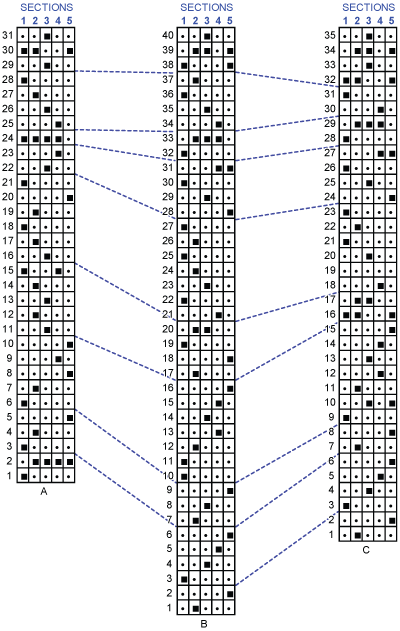
Fig. 3.B ![]() . The stratigraphic distribution of the UAs in the 5 sections is typical of a succession of transgressive � regressive cycles. The identification of successive UAs in the stratigraphic sections systematically migrate from distal to proximal sections (1 to 5) during transgressive phases and from proximal to distal (5 to 1) during regressive phases (black squares in
Fig. 3.B
. The stratigraphic distribution of the UAs in the 5 sections is typical of a succession of transgressive � regressive cycles. The identification of successive UAs in the stratigraphic sections systematically migrate from distal to proximal sections (1 to 5) during transgressive phases and from proximal to distal (5 to 1) during regressive phases (black squares in
Fig. 3.B ![]() ). The identification of trangressive-regressive cycles based on these migrations match (and partly improve) the results obtained by
(1991) and et al.
(2015) (see also , 1984). Note that using the duplicating technique described above, we get results that are very similar to the ones obtained by using the tool "Fads only" of UAgraph
(Fig. 3.C
). The identification of trangressive-regressive cycles based on these migrations match (and partly improve) the results obtained by
(1991) and et al.
(2015) (see also , 1984). Note that using the duplicating technique described above, we get results that are very similar to the ones obtained by using the tool "Fads only" of UAgraph
(Fig. 3.C ![]() ).
).
Click on thumbnail to enlarge the image.
Figure 3:
A. Reproducibility of the 31 UAs constructed on 's raw data (from ,
1991). B. Reproducibility of the different UAs 1 to 40 in sections 1 to 5 obtained after duplicating the initial data with the FOs. That diagram shows that in
Fig. 3.B ![]() the UA interval 1 to 9 is essentially transgressive and is followed by a regressive event in 10-11. A second cycle is transgressive from UA 11 to UA 18 and is followed by a regressive phase up to UA 25-27. The stability around UA 33 (UA 24 in A and 29 in
Fig. 3.C
the UA interval 1 to 9 is essentially transgressive and is followed by a regressive event in 10-11. A second cycle is transgressive from UA 11 to UA 18 and is followed by a regressive phase up to UA 25-27. The stability around UA 33 (UA 24 in A and 29 in
Fig. 3.C ![]() ) could be indicative of an accomplished transgressive phase (UA 27 to 31). A last regression followed by a final
transgression is observed between UA 34-37 (see text).
C. Reproducibility of UAs obtained by using the Fads only tool of UAgraph (details in et al.,
2015). The three diagrams show the same trends of transgressive-regressive cycles but solution B has a better resolution.
) could be indicative of an accomplished transgressive phase (UA 27 to 31). A last regression followed by a final
transgression is observed between UA 34-37 (see text).
C. Reproducibility of UAs obtained by using the Fads only tool of UAgraph (details in et al.,
2015). The three diagrams show the same trends of transgressive-regressive cycles but solution B has a better resolution.
The assemblage observed in a given sample determines the UAs to which the sample is assigned. When we observe a species or a pair of species that is exclusively restricted to one single UA, then the samples can be assigned to this and only this UA. In this case we say that the UA under consideration is strictly identified in the sample. These UAs are indicated with black squares in the reproducibility chart of the UAgraph program
(Fig. 3 ![]() ). When the fossil content of the sample does not allow the strict identification of one UA, then the sample is assigned to the union of UAs containing the smallest intersection of the fossil species observed in the sample. For visual simplicity this information is indicated with grey rectangles in the reproducibilty chart. Thanks to this procedure, one can read graphically the superpositional control between UAs and the lateral traceability of each UA.
). When the fossil content of the sample does not allow the strict identification of one UA, then the sample is assigned to the union of UAs containing the smallest intersection of the fossil species observed in the sample. For visual simplicity this information is indicated with grey rectangles in the reproducibilty chart. Thanks to this procedure, one can read graphically the superpositional control between UAs and the lateral traceability of each UA.
The application of this test to 's example
(Fig. 3 ![]() ) highlights the weak superpositional control and the poor lateral reproducibility of the different isolated UAs. As discussed below, a group of UAs without superpositional control and lateral traceability has to be grouped to make a significant zone. The relative order of these assemblages along the vertical ("time") axis of the reproducibility chart is based on the superpositions of the species which are recorded in the database (see et al.,
2015, for details). The case where the vertical distribution of unconstrained UAs migrate systematically from distal to proximal sections and inversely is controlled by the location of each section within the basin, i.e. the assemblages observed in the UAs are controlled by changing ecological conditions
(e.g., sea level fluctuations, see Figs. 3
) highlights the weak superpositional control and the poor lateral reproducibility of the different isolated UAs. As discussed below, a group of UAs without superpositional control and lateral traceability has to be grouped to make a significant zone. The relative order of these assemblages along the vertical ("time") axis of the reproducibility chart is based on the superpositions of the species which are recorded in the database (see et al.,
2015, for details). The case where the vertical distribution of unconstrained UAs migrate systematically from distal to proximal sections and inversely is controlled by the location of each section within the basin, i.e. the assemblages observed in the UAs are controlled by changing ecological conditions
(e.g., sea level fluctuations, see Figs. 3 ![]() - 4
- 4 ![]() ).
).
This holds true for UAs based on species assemblages (Fig.
3.A ![]() ), on datum only
(Fig. 3.C
), on datum only
(Fig. 3.C ![]() ) or on an augmented database
(Fig. 3.B
) or on an augmented database
(Fig. 3.B ![]() ). The addition of FOs (and/or LOs) to a given database has the advantage to increase the number of identified UAs and therefore improve considerably the readability of the reproducibility chart. In this case we can note that the datums generating new UAs are those affected by a weak diachronism.
). The addition of FOs (and/or LOs) to a given database has the advantage to increase the number of identified UAs and therefore improve considerably the readability of the reproducibility chart. In this case we can note that the datums generating new UAs are those affected by a weak diachronism.
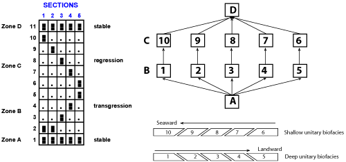
The following diagrams (Fig. 4.A-C ![]() ) shows the reproducibility of 12 imaginary UAs in a "deep to shallow" transect like that of . UAs 0 and 11 cover the whole area and are true biochronozones. UAs 1 to 5 and 6 to 10 are respectively synchronous and allow to consider their union as zones B and C. The geographic distribution of their characteristic elements is strictly controlled by the depth. In the lower cycle, the characteristic elements of the UAs are migrating landward (from left to right = transgression) and the opposite situation is represented in the regressive event (see the diagrams below). The reproducibility of the UAs can be expressed into a graph
that we have denoted as Gk' in
(1991). The last diagram of that figure explains why the variation of the indices of the UAs are oriented towards the right in the transgressive phase (zone B) and in the opposite direction in the regressive phase (zone C). The obliques cuttings of the blocks UAs 1 to 10 illustrates the origin of the inter � UAs ordering. That theoretical interpretation is based on the analysis of the variations of the indices in the sedimentary units studied by
(loc. cit.). For example the reader is referred to Fig. 5.3 of et al.,
2015 (ostracods +
foraminifera). The indices of the UAs of the first main transgressive event are organised from left to right: 6 �
7 - x - 9 -10. In the following regression the indices are organised as 15 � 14 � 13 � 14/15, followed by the next regressive event where the indices are organised as 18 � 17 � 16. However it should be noted that the above explanation has no general value because it is easy to find imaginary examples where the cycles are organized in an opposite way.
) shows the reproducibility of 12 imaginary UAs in a "deep to shallow" transect like that of . UAs 0 and 11 cover the whole area and are true biochronozones. UAs 1 to 5 and 6 to 10 are respectively synchronous and allow to consider their union as zones B and C. The geographic distribution of their characteristic elements is strictly controlled by the depth. In the lower cycle, the characteristic elements of the UAs are migrating landward (from left to right = transgression) and the opposite situation is represented in the regressive event (see the diagrams below). The reproducibility of the UAs can be expressed into a graph
that we have denoted as Gk' in
(1991). The last diagram of that figure explains why the variation of the indices of the UAs are oriented towards the right in the transgressive phase (zone B) and in the opposite direction in the regressive phase (zone C). The obliques cuttings of the blocks UAs 1 to 10 illustrates the origin of the inter � UAs ordering. That theoretical interpretation is based on the analysis of the variations of the indices in the sedimentary units studied by
(loc. cit.). For example the reader is referred to Fig. 5.3 of et al.,
2015 (ostracods +
foraminifera). The indices of the UAs of the first main transgressive event are organised from left to right: 6 �
7 - x - 9 -10. In the following regression the indices are organised as 15 � 14 � 13 � 14/15, followed by the next regressive event where the indices are organised as 18 � 17 � 16. However it should be noted that the above explanation has no general value because it is easy to find imaginary examples where the cycles are organized in an opposite way.
A general discussion of the problems related to such complex zonal interpretations is given in various chapters of the book by (1991) and will not be repeated here.
Click on thumbnail to enlarge the image.
Figure 4: Reproducibility of 12 imaginary UAs in a "deep to shallow" transect (see text), Gk' graph of the UAs represented in the reproducibility table and explanation of the individual superpositions of the UAs 1 to 10.
It is well known that the construction of zones based on "datums" (FOs or LOs) is a problem which can only be solved when a robust relative chronological framework (i.e., an order relation) based on co-occurrences has been established, allowing to know which datums are synchronous and can be used for correlations and which are diachronous and useless for direct correlations. The duplication technique described above provides an easy way to establish a sequence of non diachronous or weakly diachronous datums.
In recent sedimentary sequences (1 to 3 million years) the paleontological record is mainly restricted to first occurrences. In such cases the stratigraphers in need of a quantitative tool can use the technique of duplication described in the present paper and apply it to the non diachrounous FOs observed in the recent sediments, or, alternatively, use the "Fad only" option of UAgraph.
J.C. (1985).- The index fossil concept and its application to quantitative biostratigraphy. In: F., F.P., J.C. & W.S. (eds.), Quantitative stratigraphy.- Reidel Publishing Company, Dordrecht, p. 43�64
A.H. & P.B. (1963).- A numerical index for biostratigraphic zonation in the mid-Tertiary of the eastern Gulf.- Gulf Coast Association of Geological Societies (GCAGS) Transactions, Shreveport, vol. 13, p. 139�147.
R.D., R.H., D.M. & P.M. (2008).- Thinking outside the zone: High-resolution quantitative diatom biochronology for the Antarctic Neogene.- Palæogeography, Palæoclimatology, Palæoecology, vol. 260, nº 1-2, p. 92�121.
P.B. (1965).- Biostratigraphic correlation of the type Shubuta Member of the Yazoo Clay and Red Bluff Clay with their equivalents in southwestern Alabama.- Alabama Geological Survey Bulletin, Tuscaloosa, vol. 80, p. 1�84.
F., J. & O. (2010).- Neogene biochronology of Antarctic diatoms: A comparison between two quantitative approaches, CONOP and UAgraph.- Palæogeography, Palæoclimatology, Palæoecology, vol. 285, nº 3-4, p. 237-247.
J. (1979).- Terminologie et m�thodes de la stratigraphie moderne.- Bulletin de la Soci�t� vaudoise des Sciences naturelles, Lausanne, nº 355, vol. 74, fasc. 3, p. 169-216
J. (1987).- Corr�lations biochronologiques et Associations Unitaires.- Presses Polytechniques Romandes, Neuch�tel, 250 p.
J. (1991).- Biochronological correlations.- Springer Verlag, Berlin, 250 p.
J., F. & �. (2015).- Discrete biochronological time scales.- Springer Verlag, Berlin, 166 p.
J.E. (1970).- Binary coefficients and clustering in biostratigraphy.- Bulletin of the Geological Society America, vol. 81, nº 11, p. 3237�3252.
J.E. (1977).- Use of certain multivariate techniques in assemblage zonal biostratigraphy. In: E.G. & J.E. (eds.), Concepts and methods of biostratigraphy.- Dowden, Hutchinson and Ross Inc., Stroudsburg, p. 187�212.
R.B. (1970).- On estimating the relative biostratigraphic values of fossils.- Bulletin of the Geological Institution of the University of Uppsala, (New Series), vol. 2, p. 49�57.
S.A., J.C. & T.S. (1978).- A comparison of methods for the quantification of assemblage zones.- Computers and Geosciences, vol. 4, nº 3, p. 229�242.
W.G. (1984).- Paleogene sea level and climates USA eastern Gulf coastal plain.- Palæogeography, Palæoclimatology, Palæoecology, vol. 47, nº 3-4, p. 261�275.
1) (1965) Taxonomic database (Benthic foraminifera and ostracods): See Appendix 2B in et al., 2015.
| Number | Taxon | F / O | |
| 1 | Alabamina wilcoxensis | F | |
| 2 | Angulogerina byramensis | F | |
| 3 | Angulogerina danvillensis | F | |
| 4 | Angulogerina vicksburgensis | F | |
| 5 | Anomalina cocoaensis | F | |
| 6 | Anomalina danvillensis | F | |
| 7 | Astacolus danvillensis | F | |
| 8 | Bolivina lazanensis | F | |
| 9 | Bolivina dalli | F | |
| 10 | Bolivina gracilis | F | |
| 11 | Bolivina mississipiensis | F | |
| 12 | Bolivina retifera | F | |
| 13 | Bolivina striatellata | F | |
| 14 | Bulimina jacksonensis | F | |
| 15 | Cancris cocoaensis | F | |
| 16 | Cibicides cocoaensis | F | |
| 17 | Cibicides pippeni | F | |
| 18 | Cibicides pseudoungerianus | F | |
| 19 | Cibicides | sp.1 | F |
| 20 | "Darbyella" danvillensis | F | |
| 21 | Discorbitura dignata | F | |
| 22 | Eponides byramensis | F | |
| 23 | Eponides jacksonensis | F | |
| 24 | Eponides mariannensis | F | |
| 25 | Eponides | sp.1 | F |
| 26 | Fursenkoina dibollensis | F | |
| 27 | Guttulina problema | F | |
| 28 | Hanzawaia mississipiensis | F | |
| 29 | Hanzawaia | sp.1 | F |
| 30 | Karreriella advena | F | |
| 31 | Lankesterina frondea | F | |
| 32 | Lanticulina convergens | F | |
| 33 | Liebusella turgida | F | |
| 34 | Marginulina cocoaensis | F | |
| 35 | Massilina decorata | F | |
| 36 | Palmula caelata | F | |
| 37 | Planulina cocoaensis | F | |
| 38 | Planulina cooperensis | F | |
| 39 | Planulina lobatulus | F | |
| 40 | Pseudoclavulina cocoaensis | F | |
| 41 | Pseudogaudryina jacksonensis | F | |
| 42 | Pseudogaudryina | sp.1 | F |
| 43 | Pyrulina sp. | F | |
| 44 | Ramulina sp. | F | |
| 45 | Robulus carolinianus | F | |
| 46 | Robulus cultratus | F | |
| 47 | Robulus limbosus | F | |
| 48 | Robulus rectidorsatus | F | |
| 49 | Robulus vicksburgianus | F | |
| 50 | Saracenaria ornatula | F | |
| 51 | Sigmomorphina costifera | F | |
| 52 | Sigmomorphina jacksonensis | F | |
| 53 | Siphonina advena | F | |
| 54 | Siphonina eocenica | F | |
| 55 | Siphonina danvillensis | F | |
| 56 | Spiroloculina | sp.1 | F |
| 57 | Spiroplectammina alabamensis | F | |
| 58 | Stilostomella cocoaensis | F | |
| 59 | Stilostomella jacksonensis | F | |
| 60 | Textularia adalta | F | |
| 61 | Textularia dibollensis | F | |
| 62 | Textularia subhauerii | F | |
| 63 | Textularia tumidulum | F | |
| 64 | Textularia | sp.2 | F |
| 65 | Uvigerina cocoaensis | F | |
| 66 | Uvigerina glabrans | F | |
| 67 | Uvigerina jacksonensis | F | |
| 68 | Uvigerina topilensis | F | |
| 69 | Uvigerina vicksburgiensis | F | |
| 70 | Vaginulina lalickeri | F | |
| 71 | Vulvulina advena | F | |
| 72 | Eponides ouachitaensis | F | |
| 73 | Textularia haerii | F | |
| 74 | Subcarinata quinqueloba | F | |
| 75 | Valvulinaria octomerata | F | |
| 76 | Flabellina lanceolata | F | |
| 77 | Flabellina | sp.1 | F |
| 78 | Frondicularia tenuissima | F | |
| 79 | Anomalin bilateralis | F | |
| 80 | Discorbis cocoaensis | F | |
| 81 | Globulina alabamensis | F | |
| 82 | Globulina gibba | F | |
| 83 | Globulina inaequalis | F | |
| 84 | Guttulina irregularis | F | |
| 85 | Hanzawaia | sp.2 | F |
| 86 | Liebusella byramensis | F | |
| 87 | Marginulina hantkeni | F | |
| 88 | Marginulina mulitplicata | F | |
| 89 | Eponides obesa | F | |
| 90 | Robulus inusitatus | F | |
| 91 | Saracenaria hantkeni | F | |
| 92 | Spiroplectammina mississipiensis | F | |
| 93 | Textularia porrecta | F | |
| 94 | Textularia | sp.1 | F |
| 95 | Uvigerina dumblei | F | |
| 96 | Uvigerina gardnerae | F | |
| 97 | Globobulimina ovata | F | |
| 98 | Rectoglandulina ovata | F | |
| 99 | Angulogerina | sp.1 | F |
| 100 | Asterigerina gallowayi | F | |
| 101 | Acanthocythereis | n.sp.1 | O |
| 102 | Actinocythereis dacyi | O | |
| 103 | Actinocythereis gibsonensis | O | |
| 104 | Actinocythereis | n.sp.1 | O |
| 105 | Actinocythereis | n.sp.2 | O |
| 106 | Ambocythere | n.sp.1 | O |
| 107 | Argilloecia hiwanneensis | O | |
| 108 | Bairdia | sp.1 | O |
| 109 | Bairdopillata ocalana | O | |
| 110 | Brachycythere mississippiensis | O | |
| 111 | Buntonia israelskyi | O | |
| 112 | Buntonia | n.sp.1 | O |
| 113 | Bythocypris gibsonensis | O | |
| 114 | Clithrocytheridea caldwellensis | O | |
| 115 | Clithrocytheridea garretti | O | |
| 116 | Clithrocytheridea grigsbyi | O | |
| 117 | Cushmanidea | n.sp.1 | O |
| 118 | Cyamocytheridea watervalleyensis | O | |
| 119 | "Cythereis" dohmi | O | |
| 120 | "Cythereis" hysonensis | O | |
| 121 | Cytherella sp.1 | O | |
| 122 | Cytherelloidea cocoaensis | O | |
| 123 | Cytheretta jacksonensis | O | |
| 124 | Cytheropteron danvillensis | O | |
| 125 | Digmocythere russelli | O | |
| 126 | Digmocythere watervalleyensis | O | |
| 127 | Echinocythereis jacksonensis | O | |
| 128 | Echinocythereis mcguirti | O | |
| 129 | Eucythere woodwardensis | O | |
| 130 | Haplocytheridea ehlersi | O | |
| 131 | Haplocytheridea montgomeryensis | O | |
| 132 | Haplocytheridea | n.sp.1 | O |
| 133 | Hemicythere kniffeni | O | |
| 134 | Henryhowella florienensis | O | |
| 135 | Isocythereis couleycreekensis | O | |
| 136 | Jugosocythereis bicarinata | O | |
| 137 | Jugosocythereis vicksburgensis | O | |
| 138 | Konarocythere spurgeonae | O | |
| 139 | Krithe hiwanneensis | O | |
| 140 | Krithe | n.sp.1 | O |
| 141 | Loxoconcha concentrica | O | |
| 142 | Loxoconcha creolensis | O | |
| 143 | n.gen.n.sp.1 | O | |
| 144 | Occultocythereis broussardi | O | |
| 145 | Paracypris rosefieldensis | O | |
| 146 | Paracytheridea belhavenensis | O | |
| 147 | Paracytheridea woodwardensis | O | |
| 148 | Propontocypris mississippiensis | O | |
| 149 | Pteryogocythereis ivani | O | |
| 150 | Pteryogocythereis murrayi | O | |
| 151 | Trachyleberidea blanpiedi | O | |
| 152 | Trachyleberis montgomeryensis | O | |
| 153 | Trachyleberis | n.sp.1 | O |
| 154 | Trachyleberis | n.sp.2 | O |
| 155 | Triginglymus | n.sp.1 | O |
2) Stratigraphic database: see appendix 2C in et al., 2015.
|
|
|
|||||||||||||||||||||||||||||||||||||||||||||||||||||||||||||||||||||||||||||||||||||||||||||||||||||||||||||||||||||||||||||||||||||||||||||||||||||||||||||||||||||||||||||||||||||||||||||||||||||||||||||||||||||||||||||||||||||||||||||||||||||||||||||||||||||||||||||||||||||||||||||||||||||||||||||||||||||||||||||||||||||||||||||||||||||||||||||||||||||||||||||||||||||||||||||||||||||||||||||||||||||||||||||||||||||||||||||||||||||||||||||||||||||||||||||||||||||||||||||||||||||||||||||||||||||||||||||||||||||||||||||||||||||||||||||||||||||||||||||||||||||||||||||||||||||||||||||||||||||||||||||||||||||||||||||||||||||||||||||||||||||||||||||||||||||||||||||||||||||||||||||||||||||||||||||||||||||||||||||||||||||||||||||||||||||||||||||||||||||||||||||||||||||||||||||||||||||||||||||||||||||||||||||||||||||||||||||||||||||||||||||||||||||||||||||||||||||||||||||||||||||||||||||||||||||||||||||||||||||||||||||||||||||||||||||||||||||||||||||||||||||||||||||||||||||||||||||||||||||
|
|
||||||||||||||||||||||||||||||||||||||||||||||||||||||||||||||||||||||||||||||||||||||||||||||||||||||||||||||||||||||||||||||||||||||||||||||||||||||||||||||||||||||||||||||||||||||||||||||||||||||||||||||||||||||||||||||||||||||||||||||||||||||||||||||||||||||||||||||||||||||||||||||||||||||||||||||||||||||||||||||||||||||||||||||||||||||||||||||||||||||||||||||||||||||||||||||||||||||||||||||||||||||||||||||||||||||||||||||||||||||||||||||||||||||||||||||||||||||||||||||||||||||||||||||||||||||||||||||||||||||||||||||||||||||||||||||||||||||||||||||||||||||||||||||||||||||||||||||||||||||||||||||||||||||||||||||||||||||||||||||||||||||||||||||||||||||||||||||||||||||||||||||||||||||||||||||||||||||||||||||||||||||||||||||||||||||||||||||||||||||||||||||||||||||||||||||||||||||||||||||||||||||||||||||||||||||||||||||||||||||||||||||||||||||||||||||||||||||||||||||||||||||||||||||||||||||||||||||||||||||||||||||||||||||||||||||||||||||||||||||||||||||||||||||||||||||||||||||||||||||