◄ Carnets Geol. 17 (3) ►
![]()
Contents
[1. Introduction]
[2. Material and methods]
[3. The allochems (larger than 0.250 mm)]
[4. The facies]
[5. Some notes on "algae"]
[6. Discussion and conclusions]
[Bibliographic references] [Appendix]
and ... [Plates]
D�pt. STU, Fac. Sci. Tech., UBO, 6 avenue Le Gorgeu, CS 93837, F-29238 Brest (France)
Department of Ecology and Evolutionary Biology,
The University of Kansas, 1200 Sunnyside Avenue, Lawrence, Kansas 66045 (USA)
TOTAL
E&P, Geo-Technology Solutions, Office BA2019, TOTAL - CSTJF, avenue
Larribau, 64018 Pau (France)
Published online in final form (pdf) on June 25,
2017
DOI 10.4267/2042/62267
[Editor: Michel Moullade; language editor:
Phil Salvador; technical editor: Bruno Granier]
![]()
Eight
macrofacies types (5) plus subtypes (3) were identified while measuring sections
along the Mussafah channel profile. These include:
� aeolian sands,
� microbial mat and microbial-laminated sediments,
� gypsum and enterolithic anhydrite, i.e.,
a diagenetic variation of the previous facies,
� muds with small pelecypods, and � its seagrass meadow version,
� Potamid sands, and � its cemented version, i.e.,
the Potamid beach-rock,
� washover fan coquina.
A complete set of analyses, including granulometry, mineral composition, clay composition, TOC, and identification of the allochems and the microfossils, was performed on this material. The facies and their genetic setting, i.e., the sequence of facies, provide a perspective on both the environmental and stratigraphical significance of their distribution, both lateral and vertical, and an example of the application of the Walther's law. The lower microbial mat is the mark of a transgression whereas the upper microbial mat is the mark of a forced regression. In conclusion, the sequence of facies allows identification of the last Holocene transgressive-regressive cycle that includes a forced regression, which probably dates back to 6,000 years BP.
� Holocene;
� Flandrian;
� Abu Dhabi;
� Persian Gulf;
� facies;
� transgression;
� forced regression.
Granier B. & Boichard R. (2017).- Sedimentological investigation on Holocene deposits in the Mussafah channel (Abu Dhabi, United Arab Emirates).- Carnets Geol., Madrid, vol. 17, no. 3, p. 39-104.
Recherches s�dimentologiques sur des
d�p�ts holoc�nes dans le canal de Mussafah (Abou Dabi, Émirats Arabes Unis).- Huit
macrofaci�s (5 types et 3 sous-types) ont �t� reconnus au cours de lev�s de
coupes s�ri�es le long du canal de Mussafah et dans son prolongement. Il
s'agit :
� de sables �oliens,
� du tapis microbien et des s�diments � laminations microbiennes associ�s,
� de gypse et d'anhydrite ent�rolithique, soit une variante diag�n�tique du
faci�s pr�c�dent,
� de boues � petits bivalves et � de sa version d'herbier marin,
� de sables � Potamides et � de leur version ciment�e, soit le gr�s de
plage � Potamides,
� de lumachelles de d�p�ts de d�bordement.
Un ensemble complet d'analyses, comprenant granulom�trie, composition min�ralogique, fraction argileuse, COT, identification des microfossiles et autres �l�ments figur�s, a �t� r�alis� sur ce mat�riel. Les faci�s et leur cadre g�n�tique, c'est-�-dire la s�quence de faci�s, donnent une id�e de l'importance � la fois environnementale et stratigraphique de leur r�partition, � la fois lat�ralement et verticalement, et fournissent un exemple d'utilisation de la loi de Walther. Le tapis microbien inf�rieur est la marque d'une transgression alors que le tapis microbien sup�rieur appara�t comme celle d'une r�gression forc�e. En conclusion, la s�quence de faci�s permet d'identifier le dernier cycle transgressif-r�gressif holoc�ne qui comprend une r�gression forc�e d�butant probablement vers 6000 ans avant J.C.
� Holoc�ne ;
� Flandrien ;
� Abou Dabi ;
� Golfe persique ;
� faci�s ;
� transgression ;
� r�gression forc�e.
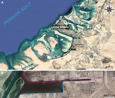
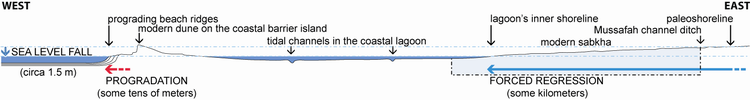
The
Mussafah channel is located on the south-eastern side of Khor Qirqishan, the
lagoon bordering the Abu Dhabi city island on its south-western side (Fig. 1 ![]() ).
This entirely artificial structure was cut inland in 1985 over a distance of
some six kilometers almost perpendicular to the coastline, i.e., in a roughly East-West direction.
).
This entirely artificial structure was cut inland in 1985 over a distance of
some six kilometers almost perpendicular to the coastline, i.e., in a roughly East-West direction.
|
Figure 1:
A)
Location (satellite image) of the Mussafah channel, Abu Dhabi (Images � 2016
TerraMetrics, Donn�es cartographiques � Google). B) Enlargement of the orange
rectangle with the red dotted contour of the channel in 1987 and its blue full
contour in 2016. |
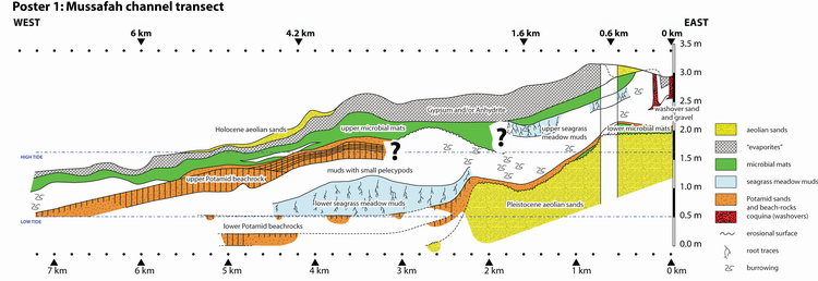
The
Mussafah channel transect (Poster 1 ![]() ) has been reconstructed from partial
sections distributed over a total length of some seven kilometers along the
channel or on its axial projection. These sections were examined in 1986 and
1987. They are two hundred meters apart on average and are identified on the
basis of their distance from the beginning of the transect along the channel
(Poster 1
) has been reconstructed from partial
sections distributed over a total length of some seven kilometers along the
channel or on its axial projection. These sections were examined in 1986 and
1987. They are two hundred meters apart on average and are identified on the
basis of their distance from the beginning of the transect along the channel
(Poster 1 ![]() ).
).
|
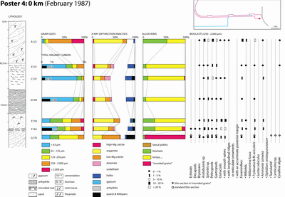
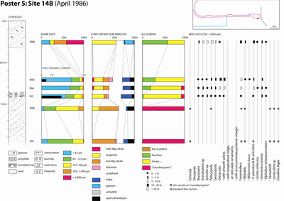
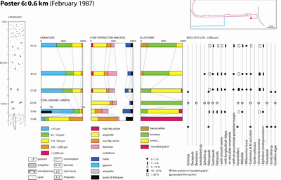
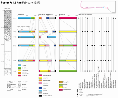
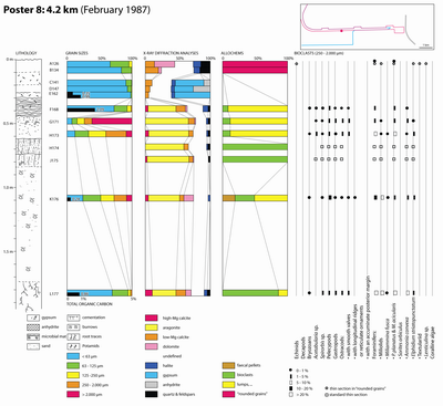
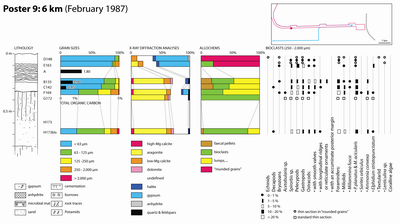
A preliminary (unpublished) TOTAL internal report was issued the next year (Granier, 1988) followed by Kenig's PhD thesis (1991) and a set of works that focus on the distribution of organic matter in the Holocene sediments of Abu Dhabi (Kenig et al., 1990; Baltzer et al., 1994; Kenig, 2011). Six of the studied sections were examined in greater detail, involving sediment sampling. They correspond to -2 km, 0 km, 0.6 km, 1.6 km, 4.2 km, and 6 km marks. Field information gathered in this study is supplemented by data from two additional sections (sites 14 B and 14 D), visited in an earlier excursion in 1986, and from a trench dug two kilometers downdip of the western end of the channel. The studied sections are:
|
|||
|
|||
|
|||
|
|||
|
|||
|
|||
|
|||
|
Most depositional facies observed along the Holocene Mussafah channel transect are currently observed on the coastal margins of the inner lagoonal areas of Abu Dhabi island where they are roughtly arranged in "living" facies belts, as recorded in the literature (e.g., Kendall & Skipwith, 1969a, 1969b; Evans et al., 1973; Alsharhan & Kendall, 2003). The few remaining facies correspond to the fossil or diagenetic counterparts of modern facies. Using an approach similar to that of Wagner and van der Togt (1973), a complete set of simple analyses (including microfacies analyses) was then run to help identifying the primary depositional macrofacies. The reconstruction of the horizontal and vertical sequence of facies enabled us to partly unravel of the last Holocene sedimentary cycle in the area studied.
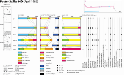
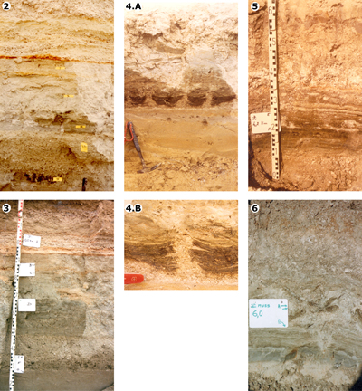
Figure 2: Site 14 D.
Figure 3: 0 km mark. Figure 4:
A) Site 14 B; B) Detail of the lower microbial mat at site 14 B.
Figure 5: 4.2 km mark.
Figure 6: 6 km mark. |
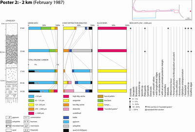
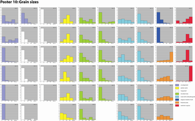
More than sixty unconsolidated samples were weighed before wet sieving and splitting into four grain size categories:
For
each sample all of these categories were dried, then weighted. The results are
expressed as a percentage of the original dry weight of the sample (Table
1; Poster 10 ![]() ). The value for a fifth category that groups all those particles finer
than 63 �m, e.g., lime mud, clay
minerals, organic matter, or sulphate salts, was back-calculated from the
difference between the above summation and the original dry weight.
). The value for a fifth category that groups all those particles finer
than 63 �m, e.g., lime mud, clay
minerals, organic matter, or sulphate salts, was back-calculated from the
difference between the above summation and the original dry weight.
Table 1: Grain sizes (%).
| Stops | Sample no. | > 2,000 �m | 250-2,000 �m | 125-250 �m | 63-125 �m |
| 14B-I | ABA 93 | 0.0 | 4.9 | 19.3 | 19.6 |
| 14B-II | ABA 94 | 0.3 | 3.1 | 5.7 | 22.6 |
| 14B-III | ABA 95 | 2.5 | 2.5 | 5.6 | 19.3 |
| 14B-IV | ABA 96 | 0.0 | 12.9 | 52.9 | 29.4 |
| 14B-V | ABA 97 | 0.0 | 1.7 | 24.3 | 59.0 |
| 14B-VI | ABA 98 | 41.7 | 28.9 | 9.4 | 2.4 |
| 14D-I | ABA 99 | 2.7 | 24.1 | 10.8 | 12.7 |
| 14D-II | ABA 100 | 0.3 | 1.2 | 2.0 | 11.1 |
| 14D-III | ABA 101 | 0.0 | 2.6 | 12.3 | 29.2 |
| 14D-IIIDis | ABA 102 | 17.5 | 25.6 | 25.1 | 18.3 |
| 14D-IV | ABA 103 | 0.8 | 11.5 | 18.6 | 20.5 |
| 14D-V | ABA 104 | 0.0 | 15.3 | 55.3 | 22.3 |
| 14E-I | ABA 105 | 0.0 | 0.1 | 0.1 | 2.4 |
| 14E-II | ABA 106 | 0.0 | 0.0 | 0.1 | 0.9 |
| 14E-III | ABA 107 | 0.0 | 0.6 | 0.7 | 5.7 |
| 14E- | ABA 110 | 0.7 | 1.8 | 2.5 | 6.0 |
| 0 km-A | ABA 121 | 28.6 | 53.9 | 9.3 | 3.4 |
| 0.2 km-A | ABA 122 | 25.7 | 13.3 | 18.1 | 5.3 |
| 0.6 km-A | ABA 123 | 0.1 | 1.8 | 23.8 | 37.1 |
| 1.6 km-A | ABA 124 | 0.0 | 2.6 | 4.8 | 17.3 |
| 4.2 km-A | ABA 126 | 0.0 | 0.3 | 4.5 | 29.8 |
| 0.2 km-A1 | ABA 127 | 7.3 | 75.2 | 12.2 | 2.3 |
| 0.2 km-A2 | ABA 128 | 94.2 | 1.7 | 1.0 | 0.9 |
| -2 km-A | ABA 129 | 12.0 | 9.6 | 2.7 | 6.6 |
| 0 km-B | ABA 131 | 0.4 | 18.1 | 9.6 | 14.7 |
| 0.6 km-B | ABA 132 | 0.1 | 4.0 | 16.9 | 18.7 |
| 1.6 km-B | ABA 133 | 2.6 | 15.8 | 3.8 | 11.6 |
| 4.2 km-B | ABA 134 | 0.0 | 0.1 | 0.9 | 15.8 |
| 6.0 km-B | ABA 135 | 0.0 | 2.2 | 5.0 | 19.3 |
| -2 km-B | ABA 136 | 0.0 | 3.9 | 1.2 | 6.9 |
| 0 km-C | ABA 137 | 0.0 | 2.3 | 3.1 | 11.5 |
| 0.6 km-C | ABA 139 | 0.0 | 4.4 | 19.9 | 24.7 |
| 1.6 km-C | ABA 140 | 0.3 | 0.1 | 0.2 | 4.6 |
| 4.2 km-C | ABA 141 | 0.0 | 0.0 | 0.5 | 9.1 |
| 6.0 km-C | ABA 142 | 0.0 | 2.3 | 5.7 | 22.7 |
| -2 km-C | ABA 143 | 0.6 | 4.7 | 1.3 | 3.4 |
| 0 km-D | ABA 144 | 1.3 | 5.2 | 6.0 | 14.1 |
| 1.6 km-D | ABA 146 | 0.2 | 2.1 | 11.5 | 20.2 |
| 4.2 km-D | ABA 147 | 0.0 | 0.0 | 1.5 | 6.8 |
| 6.0 km-D | ABA 148 | 0.0 | 0.8 | 0.4 | 6.6 |
| -2 km-D | ABA 149 | 0.0 | 2.7 | 4.6 | 22.1 |
| 0 km-E | ABA 150 | 8.0 | 22.4 | 21.5 | 29.0 |
| 1.6 km-E | ABA 161 | 10.9 | 29.5 | 14.7 | 17.8 |
| 4.2 km-E | ABA 162 | 0.0 | 0.0 | 0.3 | 1.6 |
| 6.0 km-E | ABA 163 | 0.2 | 6.9 | 1.1 | 3.4 |
| -2 km-E | ABA 164 | 0.0 | 10.1 | 12.9 | 35.2 |
| 0 km-F | ABA 165 | 6.8 | 26.5 | 12.3 | 18.9 |
| 0.6 km-F | ABA 166 | 0.0 | 31.8 | 41.0 | 19.7 |
| 4.2 km-F | ABA 168 | 0.4 | 1.6 | 6.3 | 19.5 |
| 6.0 km-F | ABA 169 | 1.2 | 14.1 | 20.6 | 33.0 |
| 0 km-G | ABA 170 | 0.0 | 15.6 | 44.9 | 20.9 |
| 4.2 km-G | ABA 171 | 62.2 | 12.2 | 10.5 | 8.2 |
| 4.2 km-H | ABA 173 | 8.5 | 31.8 | 27.0 | 20.5 |
| 6.0 km-H | ABA 173bis | 3.3 | 11.1 | 10.9 | 46.4 |
| 4.2 km-K | ABA 176 | 7.5 | 19.7 | 20.3 | 28.1 |
| 4.2 km-L | ABA 177 | 0.2 | 2.2 | 3.8 | 23.9 |
|
Finally, discrete allochem types ranging in size from 0.250 to 2 mm were identified using stereoscopic lenses and their proportion of the total population expressed as a percentage (Table 2). By comparison, Wagner and van der Togt (1973) were only considering three categories (finer than 63 �m, between 63 �m and 2 mm, larger than 2 mm).
Table 2: Components (250 -2,000 �m).
 |
||||||||||||||||||||||||||||
| 14B-I | ABA 93 | - | - | 1 | - | - | - | - | 1 | - | 1 | - | 91 | 6 | ||||||||||||||
| 14B-II | ABA 94 | - | 2 | 1 | 2 | 1 | 7 | 7 | 8 | 6 | - | 2 | - | 72 | 7 | |||||||||||||
| 14B-III | ABA 95 | - | - | - | 3 | 2 | 17 | 17 | 6 | - | - | 4 | 2 | 68 | 1 | |||||||||||||
| 14B-IV | ABA 96 | X | X | X | X | X | X | X | X | 100 | ■ | |||||||||||||||||
| 14B-V | ABA 97 | X | X | X | X | X | X | X | X | X | 100 | ■ | ||||||||||||||||
| 14B-VI | ABA 98 | 3 | 10 | 8 | 21 | 6 | - | - | 14 | 1 | 11 | - | 1 | - | 38 | 1 | ■ | |||||||||||
| 14D-I | ABA 99 | - | - | - | - | - | - | 100 | ||||||||||||||||||||
| 14D-II | ABA 100 | 4 | 2 | 1 | - | - | 1 | - | - | - | 76 | 13 | - | |||||||||||||||
| 14D-III | ABA 101 | 2 | - | 3 | - | 2 | 2 | 2 | 2 | - | 80 | 11 | ||||||||||||||||
| 14D-IIIDis | ABA 102 | - | 8 | 2 | 3 | 2 | 17 | 17 | 2 | 2 | - | 66 | ||||||||||||||||
| 14D-IV | ABA 103 | - | 6 | 4 | 3 | 3 | 2 | 2 | 2 | 2 | 80 | |||||||||||||||||
| 14D-V | ABA 104 | X | * | * | * | - | - | - | * | X | * | X | X | X | X | 100 | ■ | |||||||||||
| 0 km-A | ABA 121 | - | 11 | 6 | 19 | 8 | - | - | - | - | 12 | 2 | 9 | 1 | 43 | |||||||||||||
| 0.6 km-A | ABA 123 | 26 | 3 | 8 | 6 | 1 | 1 | 30 | 1 | - | 5 | 20 | 3 | 17 | 14 | 14 | ||||||||||||
| 1.6 km-A | ABA 124 | * | - | X | * | X | X | X | X | 100 | ■ | |||||||||||||||||
| 4.2 km-A | ABA 126 | X | X | X | X | X | X | X | 100 | ■ | ||||||||||||||||||
| -2 km-A | ABA 129 | 100 | ■ | |||||||||||||||||||||||||
| 0 km-B | ABA 131 | - | 1 | 1 | 2 | 2 | 1 | - | - | - | - | 93 | ||||||||||||||||
| 0.6 km-B | ABA 132 | - | 39 | - | 1 | 1 | - | - | 23 | - | - | - | 19 | 4 | 32 | 5 | 5 | |||||||||||
| 1.6 km-B | ABA 133 | - | - | - | - | - | - | - | - | - | - | 100 | - | |||||||||||||||
| 4.2 km-B | ABA 134 | X | x | X | X | X | X | X | 100 | ■ | ||||||||||||||||||
| 6.0 km-B | ABA 135 | - | 4 | 3 | 3 | 10 | 8 | 1 | 1 | 18 | - | 17 | - | 62 | ||||||||||||||
| -2 km-B | ABA 136 | 100 | ■ | |||||||||||||||||||||||||
| 0 km-C | ABA 137 | 1 | 1 | 7 | 1 | - | - | 2 | 2 | 86 | 2 | |||||||||||||||||
| 0.6 km-C | ABA 139 | 7 | - | 2 | 2 | - | - | 15 | - | - | 13 | 2 | 74 | 2 | 2 | |||||||||||||
| 6.0 km-C | ABA 142 | - | 3 | 6 | 2 | 3 | 3 | - | 14 | 1 | - | 11 | 2 | 54 | 18 | |||||||||||||
| -2 km-C | ABA 143 | X | X | 100 | ■ | |||||||||||||||||||||||
| 0 km-D | ABA 144 | - | 3 | - | - | - | - | 96 | ||||||||||||||||||||
| 0.6 km-D | ABA 145 | X | X | X | X | X | X | X | X | X | X | X | X | ■ | ||||||||||||||
| 1.6 km-D | ABA 146 | - | 3 | - | 1 | 1 | 52 | 1 | - | - | 45 | 4 | 22 | 23 | ||||||||||||||
| 4.2 km-D | ABA 147 | X | X | X | ■ | |||||||||||||||||||||||
| 6.0 km-D | ABA 148 | X | X | - | * | * | - | - | * | X | - | X | X | X | 100 | ■ | ||||||||||||
| -2 km-D | ABA 149 | X | X | X | X | X | X | X | X | X | 100 | ■ | ||||||||||||||||
| 0 km-E | ABA 150 | 3 | 2 | 1 | 2 | 15 | 15 | 4 | - | 1 | 3 | 73 | ||||||||||||||||
| 0.6 km-E | ABA 160 | 3 | 3 | 3 | 3 | - | 6 | - | 5 | - | 77 | 8 | ||||||||||||||||
| 1.6 km-E | ABA 161 | - | 6 | 2 | 11 | 1 | - | - | - | - | 16 | 2 | - | 10 | 4 | - | 60 | 3 | ||||||||||
| 6.0 km-E | ABA 163 | X | X | 2 | 10 | 6 | - | - | 2 | - | * | 2 | X | X | 80 | ■ | ||||||||||||
| -2 km-E | ABA 164 | X | X | X | X | X | X | X | X | X | X | 100 | ||||||||||||||||
| 0 km-F | ABA 165 | - | - | - | 10 | 4 | - | 1 | 8 | 8 | 4 | - | 2 | 2 | 64 | 8 | ||||||||||||
| 0.6 km-F | ABA 166 | X | X | X | X | X | X | X | 100 | ■ | ||||||||||||||||||
| 1.6 km-F | ABA 167 | X | X | X | X | X | X | X | X | X | X | X | X | ■ | ||||||||||||||
| 4.2 km-F | ABA 168 | - | - | - | 3 | - | - | - | 2 | 1 | - | 90 | ||||||||||||||||
| 6.0 km-F | ABA 169 | - | 1 | 6 | 7 | 2 | - | - | 21 | 2 | - | 17 | - | 2 | - | 42 | 21 | |||||||||||
| 0 km-G | ABA 170 | * | * | 1 | - | * | * | 3 | 3 | - | * | X | X | X | - | 96 | ■ | |||||||||||
| 4.2 km-G | ABA 171 | * | - | 2 | 1 | 3 | 3 | 4 | * | 3 | 1 | * | 88 | ■ | ||||||||||||||
| 6.0 km-I | ABA 172 | X | X | X | X | X | X | X | X | X | X | X | ■ | |||||||||||||||
| 4.2 km-H | ABA 173 | - | 1 | 2 | - | 1 | 1 | 8 | - | - | 6 | - | 1 | 87 | - | |||||||||||||
| 6.0 km-H | ABA 173bis | - | 6 | 35 | 5 | 3 | 3 | - | 28 | 8 | - | 15 | 1 | 3 | 19 | 4 | ||||||||||||
| 4.2 km-I | ABA 174 | X | X | X | X | X | X | X | X | X | X | ■ | ||||||||||||||||
| 4.2 km-J | ABA 175 | X | X | X | X | X | X | X | X | X | X | X | ■ | |||||||||||||||
| 4.2 km-K | ABA 176 | - | - | 11 | - | - | - | - | 16 | 6 | - | 4 | 3 | 3 | 49 | 21 | ||||||||||||
| 4.2 km-L | ABA 177 | - | 1 | 5 | 2 | 3 | 3 | 75 | 20 | - | 45 | 8 | 1 | 14 | - |
Lithified samples and those allochems first called "rounded grains", which were barely identifiable, may require petrographic thin sections for reliable identification. In such cases only occurrences, not percentages, are reported.
Additionally, G. Jousson analysed the mineralogical composition of the samples by X-ray diffractometers (Table 3). Identification of the clay minerals was performed on about ten samples only (Table 4). In addition, F. Kenig analysed the Total Organic Carbon (TOC) of about fifteen samples (Table 5).
All the results of these analyses are compiled in a set of tables (Tables 2 - 3 - 4 - 5).
Table 3: Mineralogical composition (%).
| Stops | Sample no. | Mg Calcite | Aragonite | Calcite | Dolomite | Halite | Gypsum | Anhydrite | K-Feldspar | Plagioclase | Quartz |
| 14B-I | ABA 93 | 0 | 27 | 6 | 5 | 26 | 0 | 0 | 0 | 0 | 6 |
| 14B-II | ABA 94 | 3 | 22 | 14 | 0 | 19 | 0 | 0 | 0 | 2 | 7 |
| 14B-III | ABA 95 | 4 | 20 | 14 | 9 | 18 | 0 | 0 | 0 | 4 | 7 |
| 14B-IV | ABA 96 | 0 | 15 | 46 | 0 | 3 | 0 | 0 | 0 | 5 | 12 |
| 14B-V | ABA 97 | 0 | 0 | 53 | 4 | 10 | 0 | 0 | 0 | 6 | 10 |
| 14B-VI | ABA 98 | 0 | 55 | 0 | 0 | 2 | 22 | 0 | 0 | 0 | 2 |
| 14D-I | ABA 99 | 4 | 39 | 6 | 5 | 15 | 0 | 0 | 0 | 0 | 3 |
| 14D-II | ABA 100 | 0 | 20 | 10 | 12 | 14 | 0 | 0 | 0 | 1 | 5 |
| 14D-III | ABA 101 | 4 | 30 | 9 | 3 | 29 | 0 | 0 | 0 | 0 | 3 |
| 14D-IIIDis | ABA 102 | 3 | 51 | 11 | 0.1 | 5 | 0 | 0 | 0 | 0 | 4 |
| 14D-IV | ABA 103 | 2 | 31 | 7 | 3 | 25 | 0 | 0 | 0 | 4 | 6 |
| 14D-V | ABA 104 | 0 | 24 | 46 | 0 | 5 | 0 | 0 | 0 | 0 | 12 |
| 0 km-A | ABA 121 | 3 | 69 | 9 | 0 | 3 | 0 | 0 | 0 | 0 | 0.1 |
| 0.2 km-A | ABA 122 | 3 | 40 | 11 | 0 | 12 | 24 | 0 | 0 | 0 | 1 |
| 0.6 km-A | ABA 123 | 4 | 33 | 10 | 8 | 13 | 0 | 0 | 0 | 0 | 4 |
| 1.6 km-A | ABA 124 | 0 | 0 | 14 | 4 | 13 | 0 | 35 | 0 | 3 | 3 |
| 3 km-A | ABA 125 | 0 | 0 | 5 | 0 | 4 | 80 | 0 | 0 | 0 | 0 |
| 4.2 km-A | ABA 126 | 0 | 0 | 14 | 31 | 12 | 0 | 0 | 4 | 3 | 7 |
| 0.2 km-A1 | ABA 127 | 0 | 58 | 8 | 0 | 1 | 0 | 0 | 0 | 2 | 2 |
| 0.2 km-A2 | ABA 128 | 0 | 70 | 5 | 0 | 1 | 0 | 0 | 0 | 0 | 2 |
| -2 km-A | ABA 129 | 0 | 0 | 5 | 33 | 14 | 0 | 0 | 3 | 2 | 3 |
| -2 km-AM | ABA 130 | 0 | 0 | 11 | 0 | 3 | 55 | 0 | 0 | 2 | 4 |
| 0 km-B | ABA 131 | 5 | 31 | 7 | 7 | 15 | 0 | 0 | 0 | 0 | 2 |
| 0.6 km-B | ABA 132 | 5 | 26 | 9 | 22 | 9 | 0 | 0 | 0 | 0 | 3 |
| 1.6 km-B | ABA 133 | 0 | 36 | 11 | 5 | 14 | 0 | 0 | 0 | 3 | 2 |
| 4.2 km-B | ABA 134 | 0 | 0 | 20 | 5 | 9 | 0 | 0 | 3 | 5 | 8 |
| 6.0 km-B | ABA 135 | 4 | 51 | 12 | 3 | 6 | 0 | 0 | 0 | 0 | 2 |
| -2 km-B | ABA 136 | 0 | 14 | 4 | 10 | 10 | 45 | 0 | 0 | 2 | 2 |
| 0 km-C | ABA 137 | 3 | 16 | 9 | 14 | 16 | 0 | 0 | 0 | 3 | 4 |
| 0.2 km-C | ABA 138 | 0 | 20 | 42 | 0 | 1 | 0 | 0 | 0 | 4 | 9 |
| 0.6 km-C | ABA 139 | 4 | 33 | 6 | 14 | 8 | 8 | 0 | 0 | 0 | 3 |
| 1.6 km-C | ABA 140 | 0 | 0 | 5 | 8 | 5 | 45 | 0.1 | 0 | 0 | 0.1 |
| 4.2 km-C | ABA 141 | 0 | 0 | 10 | 0 | 5 | 44 | 9 | 0 | 0 | 1 |
| 6.0 km-C | ABA 142 | 0 | 0 | 5 | 0 | 5 | 59 | 4 | 0 | 0 | 0 |
| -2 km-C | ABA 143 | 0 | 0 | 6 | 0 | 6 | 55 | 8 | 0 | 0 | 0 |
| 0 km-D | ABA 144 | 5 | 25 | 11 | 4 | 18 | 0 | 0 | 0 | 0 | 3 |
| 0.6 km-D | ABA 145 | 0.1 | 46 | 7 | 9 | 5 | 0 | 0 | 0 | 0 | 3 |
| 1.6 km-D | ABA 146 | 4 | 27 | 9 | 22 | 8 | 0 | 0 | 0 | 0 | 2 |
| 4.2 km-D | ABA 147 | 0 | 0 | 7 | 0 | 5 | 29 | 25 | 0.1 | 0.1 | 1 |
| 6.0 km-D | ABA 148 | 0 | 0 | 10 | 0 | 5 | 55 | 3 | 0 | 0 | 0 |
| -2 km-D | ABA 149 | 0 | 0 | 17 | 3 | 8 | 0 | 70 | 0 | 0 | 1 |
| 0 km-E | ABA 150 | 3 | 47 | 14 | 0 | 4 | 0 | 3 | 0 | 0 | 7 |
| 0.6 km-E | ABA 160 | 0 | 10 | 17 | 15 | 20 | 0 | 0 | 0 | 0 | 4 |
| 1.6 km-E | ABA 161 | 6 | 43 | 6 | 19 | 3 | 0 | 0 | 0 | 0 | 3 |
| 4.2 km-E | ABA 162 | 0 | 0 | 5 | 0 | 5 | 55 | 0.1 | 0 | 0 | 0 |
| 6.0 km-E | ABA 163 | 0 | 12 | 8 | 0 | 4 | 53 | 0 | 0 | 0 | 0 |
| -2 km-E | ABA 164 | 0 | 0 | 39 | 6 | 6 | 0 | 7 | 0 | 3 | 8 |
| 0 km-F | ABA 165 | 2 | 36 | 11 | 4 | 12 | 0 | 0 | 0 | 0 | 5 |
| 0.6 km-F | ABA 166 | 0 | 18 | 45 | 5 | 2 | 0 | 0 | 0 | 5 | 10 |
| 1.6 km-F | ABA 167 | 7 | 50 | 10 | 5 | 0.1 | 0 | 0 | 0 | 3 | 4 |
| 4.2 km-F | ABA 168 | 4 | 43 | 15 | 3 | 8 | 0 | 0 | 0 | 0 | 3 |
| 6.0 km-F | ABA 169 | 4 | 56 | 7 | 0 | 3 | 10 | 0 | 0 | 0 | 2 |
| 0 km-G | ABA 170 | 0 | 22 | 42 | 2 | 4 | 0 | 0 | 0 | 5 | 15 |
| 4.2 km-G | ABA 171 | 0 | 67 | 9 | 2 | 3 | 0 | 0 | 0 | 0 | 3 |
| 6.0 km-G | ABA 172 | 0.1 | 57 | 6 | 3 | 1 | 0 | 0 | 0 | 0 | 2 |
| 4.2 km-H | ABA 173 | 5 | 62 | 7 | 0 | 2 | 0 | 0 | 0 | 0 | 3 |
| 6.0 km-H | ABA 173bis | 5 | 55 | 8 | 4 | 1 | 0 | 0 | 0 | 0 | 2 |
| 4.2 km-I | ABA 174 | 0 | 60 | 7 | 0 | 2 | 0 | 0 | 0 | 0 | 3 |
| 4.2 km-J | ABA 175 | 3 | 65 | 6 | 2 | 0 | 0 | 0 | 0 | 0 | 2 |
| 4.2 km-K | ABA 176 | 5 | 48 | 7 | 15 | 2 | 0 | 0 | 0 | 0 | 0.1 |
| 4.2 km-L | ABA 177 | 11 | 37 | 15 | 8 | 4 | 0 | 0 | 0 | 1 | 3 |
Table 4: Clay minerals (%).
| Stops | Sample no. | kaolinite | illite | attapulgite | montmorillonite | chlorite |
| 14B-V | ABA 97 | 14 | 0 | 40 | 41 | 5 |
| 0.6 km-B | ABA 132 | 9 | 27 | 33 | 21 | 10 |
| 6.0 km-B | ABA 135 | 13 | 35 | 39 | 0 | 13 |
| 1.6 km-C | ABA 140 | 11 | 26 | 30 | 22 | 11 |
| 6.0 km-C | ABA 142 | 12 | 35 | 41 | 0 | 12 |
| 1.6 km-D | ABA 146 | 28 | 29 | 20 | 0 | 23 |
| 1.6 km-E | ABA 161 | 26 | 37 | 17 | 0 | 20 |
| 4.2 km-F | ABA 168 | 20 | 33 | 31 | 0 | 16 |
| 0 km-G | ABA 170 | 99 | 0 | 0 | 0 | 0 |
| 4.2 km-H | ABA 173 | 16 | 31 | 38 | 0 | 15 |
| 4.2 km-K | ABA 176 | 20 | 29 | 19 | 17 | 15 |
| 4.2 km-L | ABA 177 | 17 | 34 | 31 | 0 | 18 |
Table 5: Total organic carbon (%).
| Stops | Sample no. | TOC |
| 6.0 km-A | 1.80 | |
| 6.0 km-B | ABA 135 | 1.00 |
| 6.0 km-C | ABA 142 | 0.45 |
| 4.2 km-E1 | ABA 162-1 | 0.35 |
| 4.2 km-E2 | ABA 162-2 | 0.99 |
| 4.2 km-K | ABA 176 | 0.24 |
| 3.6 km-A | 1.57 | |
| 3.0 km-A | 0.00 | |
| 2.6 km-A | 1.00 | |
| 2.6 km-B | 0.58 | |
| 1.6 km-B | ABA 133 | 0.36 |
| 1.6 km-C | ABA 140 | 0.22 |
| 1.6 km-D | ABA 146 | 0.18 |
| 1.6 km-E | ABA 161 | 0.18 |
| 0.6 km-E | ABA 160 | 1.22 |
| 0.2 km-B | 0.00 | |
| 0 km-B | ABA 131 | 0.62 |
| 0 km-C | ABA 137 | 0.36 |
| 0 km-D | ABA 144 | 0.98 |
| 0 km-F | ABA 165 | 1.19 |
| -2 km-A | ABA 129 | 1.88 |
| -2 km-B | ABA 136 | 0.96 |
| -2 km-C | ABA 143 | 0.97 |
| -2 km-BL2 | 1.48 | |
| -2 km-BG1 | 0.04 | |
| -2 km-BG2 | 0.09 | |
| 0 km-RE | 2.04 | |
| 4.2 km-L | ABA 177 | 0.86 |
| 4.2 km-F | ABA 168 | 2.09 |
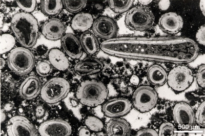
Four basic types of grains were identified: bioclasts, faecal pellets, lumps and intraclasts, and undetermined grains.
In this classification, the bioclasts comprise all skeletal remains the origin of which can still be clearly identified.
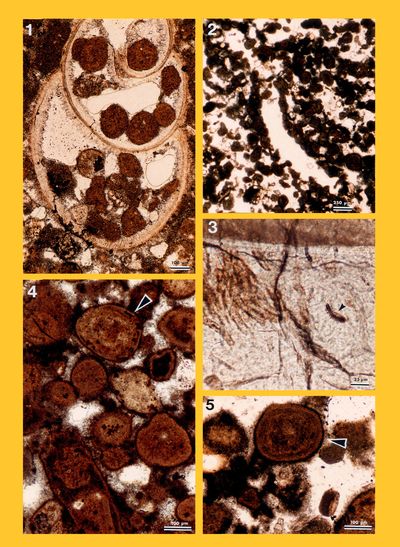
In
this material we identified some faecal
pellets with a peculiar spiral structure (Pl. 8 ![]() , fig. 5.a-d).
According to Trichet (1967), "cette figure d'h�lice serait due �
une activit� digestive pr�f�rentielle dans des zones de pression accentu�e d�termin�es
par la forme de l'intestin de l'animal" [this spiral shape may be related
to the preferential digestive activity of the animal in zones of increased
pressure determined by the morphology of its intestine]. In the same
publication, the author provides information on their mineralization, i.e.,
on the precipitation of aragonite needles within an organic matrix. In this
material dolomite rhombs grew in the needle mesh and eventually replaced the
aragonite (Pl. 8
, fig. 5.a-d).
According to Trichet (1967), "cette figure d'h�lice serait due �
une activit� digestive pr�f�rentielle dans des zones de pression accentu�e d�termin�es
par la forme de l'intestin de l'animal" [this spiral shape may be related
to the preferential digestive activity of the animal in zones of increased
pressure determined by the morphology of its intestine]. In the same
publication, the author provides information on their mineralization, i.e.,
on the precipitation of aragonite needles within an organic matrix. In this
material dolomite rhombs grew in the needle mesh and eventually replaced the
aragonite (Pl. 8 ![]() , fig. 6).
, fig. 6).
Lumps
are aggregates of grains of various types (Pl. 15 ![]() , fig. 5).
, fig. 5).
Intraclasts are by-products of in situ early lithification with a limited reworking.
"Rounded
grains"
are calcitic grains commonly eroded and centripetally micritized. A petrographic
thin section may be useful to analyse such grains. In most cases they are small
lithoclasts. We can thus identify inside them smaller allochems with calcitic
cements (Pl. 9 ![]() , figs. 1-4) and/or micritic matrices. Because all the components
of these lithoclasts are truncated at their edges we assume that they probably
result from the dismantling of layers already lithified and that they fall under
the type defined as extraclasts.
Constituent grains are commonly benthic foraminifers (e.g.,
Textulariidae: Pl. 9
, figs. 1-4) and/or micritic matrices. Because all the components
of these lithoclasts are truncated at their edges we assume that they probably
result from the dismantling of layers already lithified and that they fall under
the type defined as extraclasts.
Constituent grains are commonly benthic foraminifers (e.g.,
Textulariidae: Pl. 9 ![]() , figs. 1 & 3-4; Lenticulinidae: Pl. 9
, figs. 1 & 3-4; Lenticulinidae: Pl. 9 ![]() , figs. 5-6). Thin
sections made on these initially undetermined grains (17 thin sections) and on
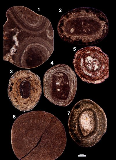
lithified samples (10 thin sections) also revealed the occurrence of ooids,
either allochthonous (reworked from Pleistocene or older rocks), calcitic with
micritic-microsparitic cortices (Pl. 10
, figs. 5-6). Thin
sections made on these initially undetermined grains (17 thin sections) and on
lithified samples (10 thin sections) also revealed the occurrence of ooids,
either allochthonous (reworked from Pleistocene or older rocks), calcitic with
micritic-microsparitic cortices (Pl. 10 ![]() , figs. 1-2, 4-5 & 7), or
autochthonous, aragonitic with micritic cortices (Pl. 11
, figs. 1-2, 4-5 & 7), or
autochthonous, aragonitic with micritic cortices (Pl. 11 ![]() , figs. 4-5). Both types
are quite different from the honey-colored ooids found in the Abu Dhabi beaches
(Pl. 10
, figs. 4-5). Both types
are quite different from the honey-colored ooids found in the Abu Dhabi beaches
(Pl. 10 ![]() , fig. 3). The mineralogical nature of these ooids was identified on thin
sections coloured with a Feigl's solution that results in a selective
colouring of the aragonite.
, fig. 3). The mineralogical nature of these ooids was identified on thin
sections coloured with a Feigl's solution that results in a selective
colouring of the aragonite.
The largest morphological and mineralogical diversity is obviously found within the bioclasts with macrofaunal (e.g., pelecypods, gastropods, echinoderms, and sponges), microfaunal (foraminifers, ostracodes, and Spirorbis) and phycological remains (Rhodophyta and Chlorophyta, e.g., Acetabularia).
Representatives
of more than ten genera of foraminifers
were identified (identifications are based on Murray, 1966,
1970, and Hottinger
et al., 1993) but some forms are
clearly older, reworked material as, for instance, large hyaline tests referred
to as Lenticulina (Pl. 9 ![]() , figs.
5-6) and agglutined tests referred to as Textulariidae (Pl. 9
, figs.
5-6) and agglutined tests referred to as Textulariidae (Pl. 9 ![]() , figs. 1 &
3-4), both found in extraclasts. The autochthonous forms comprise porcelaneous
tests:
, figs. 1 &
3-4), both found in extraclasts. The autochthonous forms comprise porcelaneous
tests:
They also comprise:
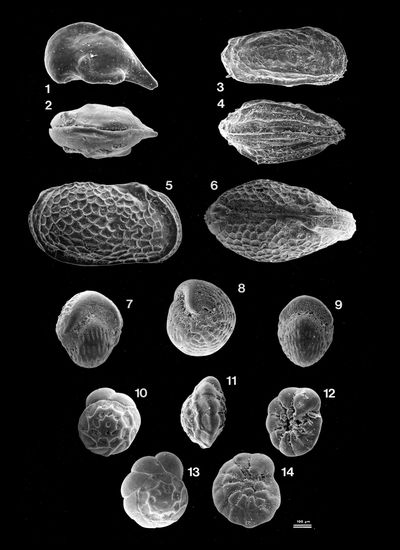
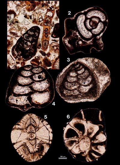
We have identified four morphotypes of ostracodes:
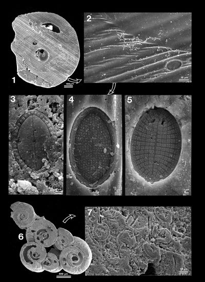
Spirorbis is an annelid characterized by its small calcareous tube, always spired
and fixed on one side (Pl. 2 ![]() , figs. 1-2, 5-7; Pl. 3
, figs. 1-2, 5-7; Pl. 3 ![]() , fig.
1; Pl. 4
, fig.
1; Pl. 4 ![]() , figs.
1 & 3). This fixing side
moulds the shape of its holder perfectly and thus offers an exact image of the
latter with its finer details (Pl. 2
, figs.
1 & 3). This fixing side
moulds the shape of its holder perfectly and thus offers an exact image of the
latter with its finer details (Pl. 2 ![]() , fig. 5; Pl. 3
, fig. 5; Pl. 3 ![]() , figs.
1-7; Pl. 4
, figs.
1-7; Pl. 4 ![]() , figs.
2 & 4).
, figs.
2 & 4).
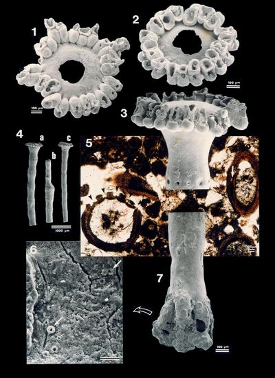
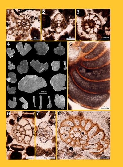
Chlorophyta
are represented by one species: Acetabularia
caliculus Lamouroux in
Quoy & Gaimard, 1824, which is still present in the area (Granier,
2012: Fig. 3.A-D). These algal remains are commonly found in the sediments in
the form of hollow aragonitic tubes corresponding to the outer calcification of
the algal thallus (Granier, 1995: Pl. 4, fig. 5-9;
2012: Fig. 5.A &
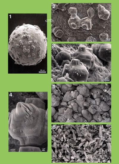
5.D; herein Pl. 1 ![]() , figs. 4.a-c & 7), and less commonly in the form of
fertile caps (Granier, 1995: Pl. 4, figs. 1-2, 4 & 10; herein Pl. 1
, figs. 4.a-c & 7), and less commonly in the form of
fertile caps (Granier, 1995: Pl. 4, figs. 1-2, 4 & 10; herein Pl. 1 ![]() ,
figs. 1-3) without fertile ampulae (Granier, 1995: Pl. 4, fig. 3). Stromengher
et al. (2010: Fig. 17.g &
17.i) misinterpreted these tubes as "worm tubes (serpulids)". Fertile ampula
are found as nuclei in some ooids (Fig. 7
,
figs. 1-3) without fertile ampulae (Granier, 1995: Pl. 4, fig. 3). Stromengher
et al. (2010: Fig. 17.g &
17.i) misinterpreted these tubes as "worm tubes (serpulids)". Fertile ampula
are found as nuclei in some ooids (Fig. 7 ![]() ). From a paleoenvironmental
perspective, Acetabularia
grows on any rigid substrate, i.e.,
on bedrocks or gravel beds, on shells (Granier, 2012: Fig. 3.A-D), and
even on larger seaweeds, seagrasses or mangrove roots. It tolerates high
salinity levels and, given its limited photosynthetic surface, it usually grows
in water depths not exceeding five meters (Dawson, 1966).
). From a paleoenvironmental
perspective, Acetabularia
grows on any rigid substrate, i.e.,
on bedrocks or gravel beds, on shells (Granier, 2012: Fig. 3.A-D), and
even on larger seaweeds, seagrasses or mangrove roots. It tolerates high
salinity levels and, given its limited photosynthetic surface, it usually grows
in water depths not exceeding five meters (Dawson, 1966).
|
Figure
7:
Fertile
ampula of a Polyphysaceae (probably an Acetabularia
sp.) as a nucleus of a Pleistocene ooid. Sample from a geotechnical core in
Pleistocene material from the Abu Dhabi offshore. |
A summary of the paleoecological preferences of the most representative benthic foraminifera (species or groups with similar paleoecological affinities) was compiled for the section studied. The information gathered includes, where available: paleobathymetry, microhabitat, oxygen preferences, temperature, and additional ecological data (Table 1). The paleoecological preferences of planktonic foraminifera with respect to surface water temperature and productivity were also summarized (Table 2).
Eight main facies types (5) and subtypes (3) were identified during field work:
4.1. The microbial mats
Occurrence of widespread microbial mats lining the intertidal flats of the Abu Dhabi emirate has been extensively described in the literature (e.g., Kendall & Skipwith, 1969a, 1969b; Evans et al., 1973; Alsharhan & Kendall, 2003).
The defining feature of this facies is the occurrence of microbial (i.e., cyanobacterial) laminae. The microbial-laminated appearance is more or less obvious depending on the ratio of organic laminae versus sedimentary laminae, on the amount of bioturbation, and the diagenetic processes among which in situ gypsum precipitation.
Granulometry:
Grains of this facies are primarily arranged into two size categories (see Poster
10 ![]() ): those where grain sizes larger than 0.250 mm represent 20 to 30 % of
the dry weight of the sediment (Samples ABA 129, 131, 133, and 165), and those
where grain sizes larger than 0.063 mm (and smaller than 0.250 mm) represent 15
to 30 % of the dry weight of the sediment (Samples ABA 135, 137, 144, and 168).
): those where grain sizes larger than 0.250 mm represent 20 to 30 % of
the dry weight of the sediment (Samples ABA 129, 131, 133, and 165), and those
where grain sizes larger than 0.063 mm (and smaller than 0.250 mm) represent 15
to 30 % of the dry weight of the sediment (Samples ABA 135, 137, 144, and 168).
Mineral composition: The microbial and the microbial-laminated sediments often contain 25 to 40 % aragonite with 5 % dolomite and 5 to 15 % calcite. However, exceptionally, some samples have mostly dolomite. This enrichment in dolomite apparently occurs to the detriment of the aragonite:
Halite presence may reach up to 30 %. Its highest percentages are always observed in these facies. Finally, both magnesian calcite and quartz are common although they never exceed 5 %.
Total Organic Carbon: The organic carbon levels of eight samples from this facies may be arranged into three groups:
Allochems ranging in size from 0.250 to 2 mm: Intraclasts commonly represent 80 to 100 % of these grain sizes whereas extraclasts and bioclasts can reach 10 % and 20 %, respectively.
The bioclasts consist of remains of pelecypods and gastropods, bryozoans, worms (Spirorbis), ostracodes (those with smooth valves), foraminifers (Peneroplis and Ammonia), and green algae (Acetabularia). Exceptionally, one sample (ABA 135 with a TOC of 1.0 %) consists of 38 % bioclasts, half of them being Peneroplis. This makes it a close match with one sample (ABA 142) from the sediment immediately underlying the microbial mat, and suggests a mixture of both facies.
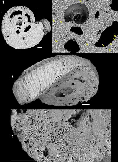
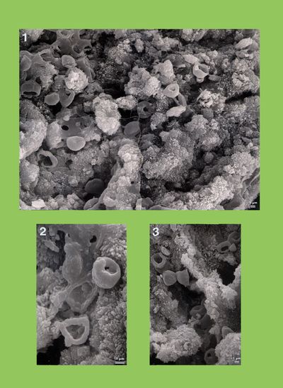
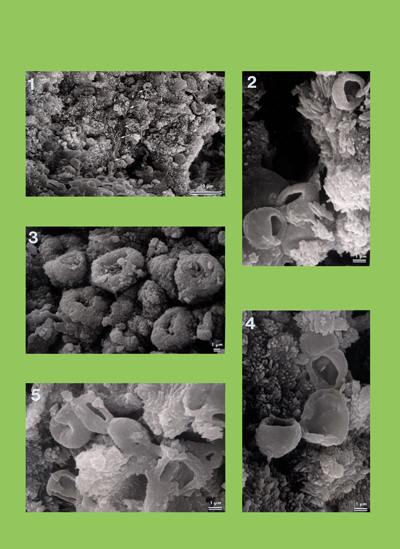
Remarks: Comparison of several diagrams of microbial mats shows that, as already pointed out by Monty (1973), their mineralisation results more from biochemical precipitation than from the incorporation of detrital grains (e.g., bioclasts). As a matter of fact, 80 to 100 % of the allochems are intraclasts, resulting from an in situ lithification. In thin section, these intraclasts consists of clotted micrite. In scanning electron microscopy (SEM), one sample (ABA 165) revealed many coccoid structures, 3 �m large in average, of cyanobacterial origin (Pls. 12-13).
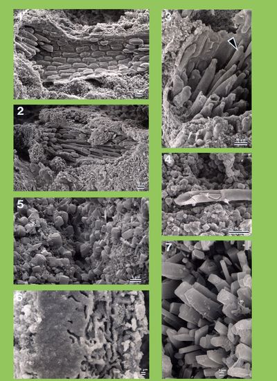
4.2. Gypsum and enterolithic anhydrite (or ? bassanite)
Similarly to the previous facies, the widespread sabkhas of the Abu Dhabi emirate have been extensively described by several authors (e.g., Kendall & Skipwith, 1969a, 1969b; Butler et al., 1982; Alsharhan & Kendall, 2003).
This facies is characterized by the abundance either of gypsum crystals of various sizes and shapes or of anhydrite in the form of enterolithic layers.
Granulometry:
As expected, particles finer than 63 �m in size, which includes the sulfate
salts, are the most prevalent in this facies (Samples ABA 124, 125, 136, 141,
143, 147, 148, 149, 162 and 163) (see Poster 10 ![]() ).
).
Mineral composition: Gypsum and anhydrite represent 45 to 70 % of the sediment. For the most part, aragonite seems to be missing, but two samples out of eleven contain slightly more than 10% (Samples ABA 136 and 163). The same generally applies to dolomite, but four samples (Samples ABA 124, 136, 140 and 149) still contain a small amount. Quartz is either missing or present at trace levels. Only calcite occurs in all the samples analysed. High-magnesian calcite is missing, but low-magnesian calcite content ranges from 5 to 15 %.
Allochems
ranging in size from 0.250 to 2 mm: They are either extraclasts or intraclasts.
Extraclasts are found in the uppermost part of the gypsum and anhydrite layer
(Samples ABA 124, 148, 149, and 163) and are thus probably of aeolian origin.
Intraclasts of this facies are found in the lowermost part of the gypsum and
anhydrite layer, next to the microbial-laminated layers (Samples ABA 130, 136,
142, 143, and 147) and therefore merely represent a diagenetic change of the
microbial mat itself (Pl. 16 ![]() ).
).
The gypsum facies is clearly a diagenetic facies (as opposed to a depositional facies). In most cases, it developed to the detriment of the microbial mat (see Monty, 1973, inter alia). Anhydrite occurred late as a replacement of gypsum as suggested by the occurrence of ghosts (i.e., pseudomorphs) of gypsum crystals and all the transitional forms to a full replacement of gypsum, as already pointed out by Illing et al. (1965).
Remark:
Gypsum may fill former intergranular pores, including locally Avicennia
mangrove roots, be present in calcareous sandy and pebbly sediments (e.g.,
samples ABA 98 or 175), and form large crystals behaving like a poecilitic
cement (Pl. 16 ![]() , fig. 2).
, fig. 2).
4.3. Muds with small pelecypods
In the field, burrows are frequently reported from this predominantly muddy facies.
Granulometry:
Besides the abundance of small pelecypods and foraminifers (Peneroplis and Ammonia),
and the activity of burrowing organisms, which are the main producers of faecal
pellets, the sediment is either a sandy to silty mud (Samples ABA 94, 132, 139,
142 and 146) or a muddy sand (Samples ABA 123, 161, 169, 173bis and 176),
eventually pebbly (see Poster 10 ![]() ).
).
Mineral composition: It is variable, apparently depending on the vertical position of the sample within the facies:
Magnesian calcite rarely exceeds 5 % (Sample ABA 177); calcite varies from 5 to 15 %. Dolomite may be missing (Samples ABA 142, 169 and 173), or may reach significant levels (i.e., up to 22 % for samples ABA 132 and 146). Quartz is always very scarce (less than 5 %). Exceptionally, one sample (ABA 142) contains 59 % gypsum.
Total Organic Carbon: The five samples analysed (ABA 142, 146, 161, 176 and 177) have values ranging between 0.2 and 0.8 %.
Allochems
ranging in size from 0.250 to 2 mm: Within this range of grain sizes there are
lumps, bioclasts and faecal pellets, which may be common (up to 5 %) or even
abundant (15-20 %). The bioclasts consist mostly of pelecypods, on the one hand,
and of foraminifers, on the other hand. The latter are Peneroplis
planatus and Ammonia
beccarii. Rather uncommon forms are exclusively or almost exclusively
found in this facies. This is particularly true for Miliammina
fusca (Brady, 1870), a Miliolidae with an agglutinated test,
and some ostracodes: Alocopocythere reticulata
indoaustralica Hartmann, 1978
(Pl. 5 ![]() , figs. 5-6),
? Cistacythereis sp. (Pl. 5
, figs. 5-6),
? Cistacythereis sp. (Pl. 5 ![]() , figs.
3-4) and Gibboborchella sp. juv.
(Pl. 5
, figs.
3-4) and Gibboborchella sp. juv.
(Pl. 5 ![]() , figs. 1-2).
, figs. 1-2).
Remark: This facies is close to the "lamellibranch mud - type no. 10" of Wagner and van der Togt (1973).
There are actually two foraminiferal subfacies: one with numerous Peneroplis and few Ammonia (samples ABA 142, 161, 169, 173, 173bis and 177) and the other inversely proportional (samples ABA 123, 132, 139 and 146) that respectively correspond to the deeper and shallower samples in the various sections studied. Thus it is highly likely that changes in the mineral composition reported above for this type of facies are largely determined by their original skeletal composition.
4.4. Seagrass meadow muds
Seagrass meadows of the Abu Dhabi lagoons are documented in the literature (e.g., Evans et al., 1973).
In the field sections, this facies is primarily distinguished from the surrounding more or less sandy and pebbly muds by the crowding of root traces and by the occurrence of Anodontia (Lucinid bivalve mollusc) shells fossilized in their living position.
Only two samples (ABA 140 -1.6 km- and ABA 177 -4.2 km-) were collected in this facies. All their key features, i.e., mineral composition (including the clay minerals), TOC, granulometry, and nature of the sand-sized allochems, significantly differ.
Remark: An additional sampling in living seagrass meadows (ABA 383, 384 and 406) suggest that there is no unique facies for seagrass meadows. These seagrasses can grow on any soft substratum, either muddy or sandy and even slightly pebbly, and do not significantly modify it. They merely introduce a subfacies that may be difficult to distinguish from the surrounding facies as there is no specific mineral, biological or organic signature (other than root tracks) for this type of environment.
4.5. Potamid sands
Occurrences of Potamid sands in the Abu Dhabi lagoons are common in the literature (e.g., Evans et al., 1973).
These calcareous sands are characterized by the abundance of Cerithideopsilla conica (Blainville, 1829), a Potamid gastropod that has a wide range of salinity tolerance from freshwater to hypersaline environments (Plaziat, 1993).
Granulometry:
70 to 80 % of the sediment consists of silt and sand (Samples ABA 102, 150 and
173) (see Poster 10 ![]() ).
).
Mineral composition: Aragonite represents 50 to 60 % of the sediments and calcite only 5 to 15 %. Dolomite is missing. Magnesian calcite, halite and quartz represent 5 % each, on average.
Clay minerals: One sample (ABA 173) was analysed. Clay minerals include 38 % attapulgite, 31 % illite, 16 % kaolinite, and 15 % chlorite.
Allochems ranging in size from 0.250 to 2 mm: They consist of bioclasts, lumps and intraclasts. The bioclasts comprise remains of gastropods and pelecypods, ostracodes (those with smooth valves), foraminifers (Peneroplis and Ammonia), and green algae (Acetabularia). The common occurrence of epiphytic faunas, such as some worm (Spirorbis) and bryozoan calcitic tests, is evidence for large seaweeds or seagrasses that were not fossilized.
Remark:
This facies is close to the "gastropod sand - type no. 6" of Wagner
and van der Togt (1973). The components of the intraclasts and lumps are bound
together by a fibrous fringing cement consisting mostly of aragonite needles
(Pl. 15 ![]() , figs. 5-6).
, figs. 5-6).
4.6. Potamid beach-rocks
Such beach-rocks are reported from areas next to Abu Dhabi island (e.g., Evans et al., 1973) and from Khor al Bazam (e.g., Alsharhan & Kendall, 2003).
These layers record early lithification. We identified at least three of them: two in a lower position and one in an upper position. However, only the upper one was sampled (ABA 145, 167, 172, 174 and 175).
Mineral composition: Aragonite represents 45 to 65 % of the sediments and calcite only 5 to 10 %. Dolomite occurs in three out of four samples and reaches a maximum of 10 %. Magnesian calcite, halite and quartz represent 5 % each, on average.
Allochems
ranging in size from 0.250 to 2 mm: These allochems are similar to the
assemblage found in the Potamid
sands, i.e., they consist of
bioclasts, lumps and intraclasts. The components of the lumps are commonly
peloids, i.e., ovoid micritic
allochems without any internal structure. Most often such grains result from the
micritization of bioclasts. Exceptionally, we also found micritic ooids in this
facies. These ooids and the peloids are both aragonitic. The primary distinction
between them is that cortices, i.e.,
concentric structures, are visible in the ooids (Pl. 11 ![]() , figs. 4-5) but are
missing in the peloids.
, figs. 4-5) but are
missing in the peloids.
Texture: The Potamid beach-rock is either a grainstone of peloidal lumps and foraminifers (less than 10 % grains larger than 2 mm) or a gastropod floatstone with grainstone matrix.
Remark:
Lithification results from cementation by radially-arranged fibers of aragonite
(Pl. 14 ![]() , fig. 7). The mineral compositions of both the Potamid
sands and the Potamid
beach-rocks are almost similar. The only difference lies in the occurrence of
dolomite in the lithified layers of the Potamid
beach-rocks. The coarse components are the same. Thus, both facies correspond to
the same depositional environment. For instance, one sample (ABA 171), the
gravel-sized allochems of which represent more than 60% of the total dry weight,
corresponds to an early stage of lithification of these Potamid
sands. The lesser or greater extent of lithification is the sole responsible for
the identification of a diagenetic subfacies: the beach-rocks.
, fig. 7). The mineral compositions of both the Potamid
sands and the Potamid
beach-rocks are almost similar. The only difference lies in the occurrence of
dolomite in the lithified layers of the Potamid
beach-rocks. The coarse components are the same. Thus, both facies correspond to
the same depositional environment. For instance, one sample (ABA 171), the
gravel-sized allochems of which represent more than 60% of the total dry weight,
corresponds to an early stage of lithification of these Potamid
sands. The lesser or greater extent of lithification is the sole responsible for
the identification of a diagenetic subfacies: the beach-rocks.
4.7. Washover fan coquina
These coarse bioclastic sands are characterized by the occurrence of a cross-bedding with low-angle laminae (5 to 10�) inclined toward the lagoon. Two coquina ridges are found in the eastern end of the Mussafah channel transect, in the first 200 meters of the transect.
Granulometry: Allochems larger than 0.250 mm (medium and coarse sands, and gravels) represent more than 60% of the total dry weight (samples ABA 98, 121, 127 and 128).
Mineral composition: Aragonite represents 55 to 70 % of the sediments and calcite never exceeds 10 %. Dolomite is missing. Magnesian calcite was identified in one sample only (ABA 121). Halite and quartz are present but they never exceed 5 % each. Exceptionally, in this facies, one sample (ABA 98) contains 22 % gypsum.
Allochems ranging in size from 0.250 to 2 mm: Bioclasts represent more than 60 % of this grain-size category. The remaining allochems are intraclasts made of more or less cemented bioclasts. On average there are 30 % of both gastropod and pelecypod shells, from 10 to 15 % foraminifers (three quarters of them are Peneroplis), 10 % Acetabularia, from 5 to 10 % Spirorbis, and up to 5 % bryozoans.
Remark: According to Reineck & Singh (1973), "the washover fan is made up of several superimposed sandy blankets of successive whashover fans (...). Each sandy blanket begins with a shell-rich layer, which possesses an erosive contact to the lower sediments. In the shelly horizon shells of macro-invertebrates from different biocenoses are mixed together. Then a sandy layer follows with well developed evenly laminated sand". That definition matches the description of the material studied, i.e., a poorly sorted assemblage of shells including Brachidontes, Tellina, Cerithium, Mitrella, Potamids, Trochidae, etc.
4.8. Aeolian sands
In the field they consist partly of a modern (uppermost Holocene) sand blanket (sample ABA 164) and partly of the Pleistocene sandy substratum.
Granulometry: Fine sand, i.e., with grain sizes ranging from 0.125 to 0.250 �m, represents from 40 to 55 % of the total dry weight for samples from the unconsolidated Pleistocene cross-bedded sands (samples ABA 96, 104, 166 and 170). Silts prevail in both the massive Pleistocene sands (sample ABA 97) and the modern aeolian blanket (sample ABA 164).
Mineral composition: This facies is characterized by the occurrence of 40 to 50 % calcite and 10 to 15 % quartz, plus 5 % feldspars, bringing the amount of siliciclastics to 15-20 %. Magnesian calcite is missing. Dolomite may reach or surpass 5 %. Halite represents 5 % in average. One sample - one of the Holocene sand (ABA 164) - contains 7 % anhydrite.
Clay minerals: Only two samples (ABA 97 and 170) were analysed for clay.
The clay mineral composition of the first sample (ABA 97), which corresponds to the finer Pleistocene sediment (silt), consists of 40 % attapulgite, 41 % montmorillonite, 14 % kaolinite, and 5 % chlorite.
The second sample (ABA 170), from the coarser Pleistocene sediment (fine sand), contains exclusively kaolinite (99 %).
As a distinguishing criterion, in relation to the other samples analysed, both samples share the absence of illite. In addition they contain very little, if any, chlorite.
Allochems ranging in size from 0.250 to 2 mm: They almost exclusively consist of "rounded grains". In petrographic thin sections, they appear to be calcitic ooids, bioclasts and extraclasts. These bioclasts are echinoid spines, various remains of gastropods and pteropods, calcareous red algae (Corallinales and Sporolithales), and foraminifers (primarily Textulariidae, Lituolidae and Lenticulinidae, and secondarily Peneroplis and forms close to Acervulinidae).
As reported above, "algae" occur in most facies. However there are some forms that we have not mentioned yet:
Coccolithophorids: Under Scanning Electron Microscopy, specimens of Miliammina, i.e., a genus ascribed to the Mililiolidae but with an agglutinated test, revealed that few coccoliths, i.e., the disc-shaped plates the assembly of which forms a coccosphere around the planktonic unicellular Haptophyta alga, are parts of the foraminiferal shell.
Diatoms: Frustules, i.e.,
the siliceous valves around Bacillariophyta unicellular algae, either
recrystallized as calcite or in the form of empty molds, were observed on the
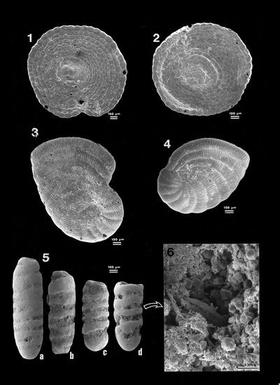
fixation face of tubes of Spirorbis (Pl. 3 ![]() , figs. 2-5 &7; Pl. 4
, figs. 2-5 &7; Pl. 4 ![]() , fig. 2). In our material, we identified pennate
forms, which have benthic life habits and commonly grow on larger algae.
, fig. 2). In our material, we identified pennate
forms, which have benthic life habits and commonly grow on larger algae.
Rhodophyta: Very few sections ascribed to Rhodophyta are observed in the
Holocene lithified samples. Hoewever, besides the diatom frustules (Pl. 3 ![]() , figs.
2-5 & 7; Pl. 4
, figs.
2-5 & 7; Pl. 4 ![]() , fig. 2), we identified Lytophyllum-like structures on the fixation face of a Spirorbis
tube (Pl. 4
, fig. 2), we identified Lytophyllum-like structures on the fixation face of a Spirorbis
tube (Pl. 4 ![]() , figs. 1-4). David M. John (personal
communication, May 6, 2017) suspects one of them "might well be" Lithophyllum
kotschyanum Unger, 1858, which "is certainly also reported
to be far the most common species elsewhere along the southern coast of the
Arabian Gulf" (see John, 2012), but he also adds it is "impossible to
be certain" from the image.
, figs. 1-4). David M. John (personal
communication, May 6, 2017) suspects one of them "might well be" Lithophyllum
kotschyanum Unger, 1858, which "is certainly also reported
to be far the most common species elsewhere along the southern coast of the
Arabian Gulf" (see John, 2012), but he also adds it is "impossible to
be certain" from the image.
In addition, Rhodophyta remains, including geniculate coralline algae
(Pl. 10 ![]() , fig. 6), are commonly found inside "rounded grains", i.e.,
inside the small Pleistocene (?) extraclasts.
, fig. 6), are commonly found inside "rounded grains", i.e.,
inside the small Pleistocene (?) extraclasts.
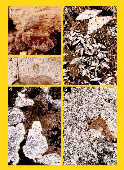
Another algal specimen observed in one sample (ABA 129) looks like red
algae, i.e.,
a pluricellular structure with pit connections (Pl. 14 ![]() , fig. 1). Brian Wysor
(personal communication, April 29, 2016) suggested it could be Bostrychia
arbuscula Harvey, 1855.
, fig. 1). Brian Wysor
(personal communication, April 29, 2016) suggested it could be Bostrychia
arbuscula Harvey, 1855.
Cyanobacteria: They are the main contributors to the microbial mats (Monty,
1973, inter alia). David M. John
(personal communication, May 13, 2016) suggested that some of our specimens (Pl. 14 ![]() , figs. 2-3) resemble interwoven filaments
of Coleofasciculus chthonoplastes
(Gomont, 1892). As is documented in our material by the intraclasts
(Pls. 12
, figs. 2-3) resemble interwoven filaments
of Coleofasciculus chthonoplastes
(Gomont, 1892). As is documented in our material by the intraclasts
(Pls. 12 ![]() - 13
- 13 ![]() ), lithification results more from biochemical precipitation processes than
from grain trapping. In association with fungi, some cyanobacteria also play a
destructive role (e.g., Rioult & Dangeard,
1976), i.e.,
bioerosion (Pl. 11
), lithification results more from biochemical precipitation processes than
from grain trapping. In association with fungi, some cyanobacteria also play a
destructive role (e.g., Rioult & Dangeard,
1976), i.e.,
bioerosion (Pl. 11 ![]() , fig. 3; Pl. 14
, fig. 3; Pl. 14 ![]() , fig. 6).
, fig. 6).
Large (brown, red or green) seaweeds: With their anchoring organs or rhizoids, they colonize either pebbly or rocky substrates. Although they are not fossilized, these forms played a considerable role in sedimentation:
Seagrasses: They are not algae, but phanerogams with roots. They commonly colonize loose, muddy or sandy, substrates. In the same way as for the large seaweeds, they form in turn the substrate of many epiphytic organisms (Beavington-Penney et al., 2004).
Among the eight facies described above, two are of diagenetic origin:
This diagenetic facies affects the uppermost half meter of sediments in
the eastern part of the transect and gets gradually thinner towards the lagoon.
It is partly controlled by the modern topography
(Poster 1 ![]() ). This type of
diagenesis affects both the Holocene aeolian sands (� 4.8.) and the microbial
mats (� 4.1.). From the lagoon up
the coastal sebkha, gypsum is gradually replaced by anhydrite. In addition, it
appears that dolomite always occurs as a replacement of aragonite, an unstable
polymorph of calcium carbonate CaCO3: see, for instance, the mineral
composition of the microbial mats and also SEM photomicrographs of faecal
pellets (e.g., Pl. 8
). This type of
diagenesis affects both the Holocene aeolian sands (� 4.8.) and the microbial
mats (� 4.1.). From the lagoon up
the coastal sebkha, gypsum is gradually replaced by anhydrite. In addition, it
appears that dolomite always occurs as a replacement of aragonite, an unstable
polymorph of calcium carbonate CaCO3: see, for instance, the mineral
composition of the microbial mats and also SEM photomicrographs of faecal
pellets (e.g., Pl. 8 ![]() , fig. 6);
, fig. 6);
They results from the early lithification of Potamid sands (�
4.5.) by aragonitic cement in a marine phreatic
setting. There are several beach-rocks clearly distinguishable on the basis of
their position and tilt
(Poster 1 ![]() ). The lower beach-rocks are partly
sub-horizontal whereas the upper beach-rock is sloping downwards toward the
lagoon.
). The lower beach-rocks are partly
sub-horizontal whereas the upper beach-rock is sloping downwards toward the
lagoon.
Furthermore the seagrass meadow muds, which are characterized by root
tracks, are merely a subfacies of the muds with small pelecypods. As already
discussed above, both facies only differ by their outer appearances: allochems,
granulometries and mineral compositions are similar. The reconstruction of the
Mussafah channel transect allows us to identify two discrete seagrass meadows
(Poster 1 ![]() ):
):
The virtual vertical sequence of facies comprises from base to top:
Although differential compaction of muds and calcareous sands due to mud
dewatering and sand cementation caused difficulties in the sequential
interpretation, three discrete sedimentary patterns have been identified in the
sequence of facies observed on the Mussafah channel transect
(Poster 1 ![]() ):
):
1) a transgressive, retrogradational, deepening upward
pattern: It starts
at a sharp contact of a relict microbial mat on the underlying Pleistocene
aeolian sands. This basal organic-rich layer is followed by Potamid
sands, then by muds with small pelecypods. The full sequence can be observed at
sections located from 0 km to 1 km from the transect origin. Beyond these
sections the basal microbial mat is missing. From 2.2 km to 4.4 km, lower
seagrass meadow muds are interposed between Potamid
sands and muds with small pelecypods. Both thick Potamid sands and seagrass
meadow sediments pinch out landward due to a topographic change between 2.0 km
and 2.4 km from the transect origin. Note that the transgression here was
probably not smooth and gradual but rather a pulsed phenomenon. The maximum of
the transgression is possibly recorded by the washover fan coquina on the
eastern (landward) side of the transect
(Poster 1 ![]() );
);
2) a regressive, progradational, shallowing upward pattern. Kenig (2011) referred to a "regressive microbial mat" but did not enter into the details regarding the sequence of events. This regressive trend is clearly divided into two parts:
2A) a normal regression. This part is not easy to characterize due to dominantly muddy facies. However, it ends locally, i.e., from 0.6 km to 1.8 km from the transect origin, with the upper seagrass meadow muds;
2B) the direct superposition of microbial mats on these upper seagrass meadow muds without interposition of Potamid sands is indicative of a significant downward shift of facies, i.e., it is the mark of a forced regression. At sections located from 3.2 km to 4.4 km from the transect origin, Potamid sands are overlain by microbial mats, which in turn are overlain by the Holocene aeolian sands. Beyond the 5.8 km mark, lagoonal muds are interposed between Potamid sands and microbial mats.
In conclusion, both microbial mats, the lower and the upper, have discrete significances in terms of relative sea-level trends. The lower microbial mat is the mark of a transgression (Kenig, 2011) whereas the upper microbial mat is the mark of a forced regression.
|
Figure 8: The model (see text for comments). |
The relative sea-level fall corresponding to this last forced regression can be estimated on the basis of the position of the upper microbial mats. It is at least 1.6 m, which is the topographic difference of these microbial maps at the 0.4 km and 7.2 km marks.
The amplitude of a transgression and that of a regression are estimated on the basis of the horizontal shifts, respectively landward and seaward, of the shoreline (i.e., the mean high water line). It can be approached through peculiar sedimentary facies found in shallow-water settings that provide evidence for water encroachment along the innermost side of the lagoon. Considering that microbial mats thrive in the upper intertidal zone, the shoreline shift during the regressive interval can be estimated soley on the basis of the location of the upper microbial mats. These upper microbial mats are found in almost all sections along the transect, starting from the - 2 km mark. Consequently, the last forced regression corresponds at least to a 5 km lateral shift, a result that is in general agreement with observations made by geologists who preceded us in the same area (Shearman, 1966, inter alia).
In the case of the Abu Dhabi lagoons, which are sited on the southern margin of an epicontinental sea, the amplitude of the progradation and that of the retrogradation in this ramp system can be estimated on the basis of the horizontal shifts, respectively lagoonward and (open) seaward, of the rollover line of the coastal oolitic barrier (i.e., the mean low water line on the open marine side of the barrier). The last forced regression led to a limited lateral seaward shift of the modern oolitic barrier in the range of some tens of meters only. The existence of the barrier and its effectiveness at protecting and isolating the lagoon have probably significantly impacted the depositional environments and the nature of the sediments in the Mussafah area during the Holocene transgressive-regressive cycle. According to some authors (Purser & Evans, 1973: Fig. 11), the coastal barrier settled on a preexisting ridge, i.e., a fossil relative high, which "has influenced all subsequent physiographic processes" (Kassler, 1973). However, further investigations on the coastal barrier and under the lagoon waters are required to test further this hypothesis.
Despite the relative incompleteness of our study, i.e.,
some subject areas have not been fully addressed and we were missing absolute
radiocarbon datings, our sedimentological analyses have documented a
transgressive-regressive sequence of facies in relation to relative sea-level
changes. Recently, Stromengher et al.
(2010) who investigated a 0.7 km long transect (compared our 9 km transect)
provided these invaluable radiocarbon ages. According to these data, the
Holocene sediments of the upper part of our transect range in age from 6,600 �
40 to 4,950 � 60 years BP (minimum range) and the youngest Pleistocene aeolian
sandstones are dated at 23,490 � 130 years BP. This information helps to better
constrain our interpretation in time. The reversal point of the relative
sea-level rise (transgression and normal regression) to the fall (forced
regression) takes place somewhere between 5,000 and 6,500 BP. That is in
agreement with several reports that places it at about 6,000 years BP
(geological reports) or at about 4,000 years BC (archaeological reports) at the "climax of the Flandrian transgression" (Barth,
2001, inter
alia). The following relative sea-level fall is estimated to be not
less than 1.5 m (1.8 m according to Kenig, 2011) with an associated
seaward shift of the shoreline of some 5 km (forced regression), whereas the
coeval seaward shift of the rollover line of the lagoon barrier might have been
of some tens of meters only (effective progradation): Fig. 8 ![]() .
.
This publication is dedicated to the memory of the late
Philippe Bousquet. The
authors would like to thank TOTAL
for having granted permission to publish this paper. Researchers participating
to the 1986 and 1987 field work were F. Baltzer, R. Boichard, M. Huc,
F. Kenig, J.-L. Oudin, J.-C. Plaziat and B. Purser.
Except for the X-ray mineralogical analyses undertaken by G. Jousson, all
laboratory analyses were conducted by B. Granier. The authors are also
very grateful to Phil Salvador who carefully polished the English text of
this manuscript, J.-C. Plaziat who provided invaluable additional
information on the coastal sedimentology of Abu Dhabi, Francesco Sciuto
who identified the ostracodes, and to David M. John, Paulo Antunes Horta,
Curt M. Pueschel, Carlos G. V�lez and Brian Wysor who
provided valuable information on some algae. SEM photos from Plate 4 ![]() were taken
by Hermes Brito at the UNESPetro, Rio Claro, SP,
Brazil.
were taken
by Hermes Brito at the UNESPetro, Rio Claro, SP,
Brazil.
Figures 9 ![]() - 10
- 10 ![]() - 11
- 11 ![]() - 12
- 12 ![]() - 13
- 13 ![]() - 14
- 14 ![]() are part of a previously unpublished contribution of Jean-Claude Plaziat.
They comprise a set of photos taken during the last field mission in February
1987.
are part of a previously unpublished contribution of Jean-Claude Plaziat.
They comprise a set of photos taken during the last field mission in February
1987.
Alsharhan A.S. & Kendall C.G.St.C. (2003).- Holocene coastal carbonates and evaporites of the southern Arabian Gulf and their ancient analogues.- Earth-Science Reviews, vol. 61, no. 3-4, p. 191-243.
Baltzer F., Kenig F., Boichard R., Plaziat J.-C. & Purser B.H. (1994).- Organic matter distribution, water circulation and dolomotization beneath the Abu Dhabi sabkha (United Arab Emirates).- International Association of Sedimentology, Special Publication, vol. 21, p. 409-427.
Barth H.-J. (2001).- Understanding of coastal fluctuation at the Arabian Gulf leading to the "lost city of Gerrha"?- Palaeoecology of Africa, vol. 27, p. 291-303.
Barth H.-J. & Khan N.Y. (2002).- Biogeophysical setting of the Gulf. In: Abuzinada A.H., Barth H.-J. , Krupp F., B�er B. & Al Abdessalaam T.Z. (eds.), Protecting the Gulf's marine ecosystems from pollution.- Birkh�user Verlag, B�le, p. 1-21.
Beavington-Penney S.J., Wright V.P. & Woelkerling W.J. (2004).- Recognising macrophyte-vegetated environments in the rock record: A new criterion using "hooked" forms of crustose coralline red algae.- Sedimentary Geology, vol. 166, p. 1-9.
Berger S. (2006).- Photo-atlas of living Dasycladales.- Carnets de G�ologie, Madrid, Book 2006/02 (CG2006_B02), ISBN 2-916733-01-9, 348 p.
Butler G.P. (1969).- Modern evaporite deposition and geochemistry of coexisting brines, the sabkha, Trucial Coast, Arabian Gulf.- Journal of Sedimentary Petrology, vol. 39, no. 1, p. 70-89.
Butler G.P., Harris P.M. & Kendall C.G.St.C. (1982).- Recent evaporites from the Abu Dhabi coastal flats. In: Deposional and diagenetic spectra of evaporites.- Core workshop, Calgary, 26-27 juin 1982.- Society of Economic Paleontologists and Mineralogists, Special Publications, Tulsa, vol. 3, p. 33-64.
Dawson E.Y. (1966).- Marine Botany.- Holt, Rinehart and Winston, New-York, 326 p.
Evans G., Kinsman D.J.J. & Shearman D.J. (1964).- A reconnaissance survey of the environment of recent carbonate sedimentation along the Trucial Coast, Persian Gulf. In: Straaten L.M.J.U. van (ed.), Deltaic and shallow marine deposits.- 6th International Sedimentological Congress, 1963.- Developments in Sedimentology, Elsevier, Amsterdam, 1, p. 129-135.
Evans G. & Kirkham A. (2002).- Part I Distribution of sabkhat within the Arabian peninsula and the adjacent countries. In: Barth H.-J. & B�er B. (eds.), Sabkha ecosystems.- Kluwer Academic Publishers, Dordrecht, p. 7-20.
Evans G., Kirkham A. & Carter R.A. (2002).- Quaternary development of the United Arab Emirates coast: New evidence from Marawah Island, Abu Dhabi.- GeoArabia, Manama, vol. 7, no. 3, p. 441-458.
Evans G., Murray J.W., Biggs H.E.J., Bate R. & Bush P.R. (1973).- The oceanography, ecology, sedimentology and geomorphology of parts of the Trucial Coast barrier island complex, Persian Gulf. In: Purser B.H. (ed.), The Persian Gulf.- Springer Verlag, Berlin, p. 233-277.
Folk R.L., Chafetz H.S. & Tiezzi P.A. (1985).- Bizarre forms of depositional and diagenetic calcite in hot-spring travertines, central Italy. In: Schneidermann N. & Harris P.M. (eds.), Carbonate cements.- Society of Economic Paleontologists and Mineralogists, Special Publications, Tulsa, vol. 36, p. 349-369.
Hottinger L., Hamicz E. & Reiss Z. (1993).- Recent Foraminiferida from the Gulf of Aqaba, Red Sea.- Slovenska akademija znanosti in umetnosti, Ljubljana, Razred za naravoslovne vede, (Classis IV: Historia naturalis), Dela * Opera, 33, 179 p. (230 Pls.).
Hughes Clarke M.W. & Keij A.J. (1973).- Organisms as producers of carbonate sediment and indicators of environment in southern Persian Gulf. In: Purser B.H. (ed.), The Persian Gulf.- Springer Verlag, Berlin, p. 33-56.
Granier B. (1988, unpublished).- �tude p�tro-s�dimentologique de la coupe du Canal de Mussafah (Abu Dhabi - �mirats Arabes Unis).- TOTAL-Compagnie Fran�aise des P�troles, Rapport Laboratoires, Pessac, no. RL 4324, 18 p.
Granier B. (1995).- The genus Actinoporella (G�mbel in Alth, 1881) and its representatives. A review. In: Proceedings of the International Symposium and Field-Meeting "Alpine Algae '93".- Beitr�ge zur Pal�ontologie, Vienna, no. 19 (1994), p. 113-127.
Granier B. (2012).- The contribution of calcareous green algae to the production of limestones: A review. In: Basso D. & Granier B. (eds.), Calcareous algae and the global change: from identification to quantification.- Geodiversitas, Paris, vol. 34, no. 1, p. 35-60.
Granier B. & Dias-Brito D. (2015).- End of a modern geological myth: there are no rudists in Brazil! Paleobiogeographic implications.- Carnets Geol., Madrid, vol. 15, no. 11, p. 123-136.
Illing L.V., Wells A.J. & Taylor J.C.M. (1965).- Penecontemporary dolomite in the Persian Gulf.- Society of Economic Paleontologists and Mineralogists, Special Publications, Tulsa, vol. 13, p. 89-11.
John D.M. (2012).- Marine algae (seaweeds) associated with coral reefs in the Gulf. In: Riegl B.M. & Purkis S.J. (eds.), Coral Reefs of the Gulf.- Coral Reefs of the World, vol. 3, p. 309-335.
Kassler P. (1973).- The structural and geomorphologic evolution of the Persian Gulf. In: Purser B.H. (ed.), The Persian Gulf.- Springer Verlag, Berlin, p. 11-32.
Kendall C.G.St.C. & Skipwith P.A. d'E. (1969a).- Holocene shallow-water carbonate and evaporite sediments of Khor al Bazam, Abu Dhabi, South-West Persian Gulf.- American Association of Petroleum Geologists, Bulletin, vol. 53, no. 4, p. 841-869.
Kendall C.G.St.C. & Skipwith P.A. d'E. (1969b).- Geormorphology of a recent shallow-water carbonate province Khor al Bazam, Trucial Coast, Southwest Persian Gulf.- Geological Society of America, Bulletin, vol. 80, no. 5, p. 865-892.
Kenig F. (1991).- S�dimentation, distribution et diag�n�se de la mati�re organique dans un environnement carbonat� hypersalin, le syst�me lagune-sabkha d'Abu Dhabi (�.A.U.).- Th�se de l'Universit� d'Orl�ans, 330 p.
Kenig F. (2011).- Distribution of organic matter in the transgressive and regressive Holocene sabkha sediments of Abu Dhabi, United Arab Emirates.- International Association of Sedimentology, Special Publication, vol. 43, p. 277-298.
Kenig F., Huc A.Y., Purser B.H. & Oudin J.-L. (1990).- Sedimentation, distribution and diagenesis of organic matter in a recent carbonate environment, Abu Dhabi, U.A.E.- Organic Geochemistry, vol. 16, no. 4-6, p. 735-747.
Kinsman D.J.J. (1964).- The recent carbonate sediment near Halat El Bahrani, Trucial Coast, Persian Gulf. In: Straaten L.M.J.U. van (ed.), Deltaic and shallow marine deposits.- 6th International Sedimentological Congress, 1963.- Developments in Sedimentology, Elsevier, Amsterdam, vol. 1, p. 185-192.
Kinsman D.J.J. (1971).- Early diagenesis of carbonate sediments in a supratidal evaporite setting.- American Association of Petroleum Geologists, Bulletin, vol. 55, no. 1, p. 167-168.
Lambeck K. (1996).- Shoreline reconstructions for the Persian Gulf since the last glacial maximum.- Earth and Planetary Science Letters, vol. 142, p. 43-57.
McKenzie J.A. (1981).- Holocene dolomitization of calcium carbonate sediments from the coastal sabkhas of Abu Dhabi, U.A.E. A stable isotope study.- Journal of Geology, Chicago, vol. 89, p. 185-198.
Monty C.L.V. (1973).- Remarques sur la nature, la morphologie et la distribution spatiale des stromatolithes. In: S�dimentation et diag�n�se des carbonates actuels.- Sciences de la Terre, Nancy, vol. 18, no. 3, p. 191-212.
Murray J.W. (1966).- The foraminifera of the Persian Gulf. 3. The Halat al Bahrani region.- Palæogeography, Palæoclimatology, Palæoecology, vol. 2, p. 59-68.
Murray J.W. (1970).- The foraminifera of the hypersaline Abu Dhabi lagoon, Persian Gulf.- Lethaia, vol. 3, no. 1, p. 51-68.
Strohmenger C.J., Al-Mansoori A., Al-Jeelani O., Al-Shamry A., Al-Hosani I., Al-Mehsin K. & Shebl H. (2010).- The sabkha sequence at Mussafah Channel (Abu Dhabi, United Arab Emirates): facies stacking patterns, microbial-mediated dolomite and evaporite overprint.- GeoArabia, vol. 15, no. 1, p. 49-90.
Patterson R.J. & Kinsman D.J.J. (1982).- Formation of diagenetic dolomite in coastal sabkha along Arabian (Persian) Gulf.- American Association of Petroleum Geologists, Bulletin, vol. 66, no. 1, p. 28-43.
Plaziat J.-C. (1993).- Modern and fossil Potamids (Gastropoda) in saline lakes.- Journal of Paleolimnology, vol. 8, no. 2, p. 163-169.
Purser B.H. & Evans G. (1973).- Regional sedimentation along the Trucial Coast, SE Persian Gulf. In: Purser B.H. (ed.), The Persian Gulf.- Springer Verlag, Berlin, p. 211-231.
Reineck H.E. & Singh I.B. (1973).- Depositional sedimentary environments.- Springer Verlag, Berlin, 439 p.
Rioult M. & Dangeard L. (1976).- Importance des Cryptogames perforantes marines en g�ologie. In: Travaux de biologie v�g�tale d�di�s au Professeur P. Dangeard.- Le Botaniste, Caen, (L), p. 389-413.
Shearman D.J. (1966).- Origin of marine evaporite by diagenesis.- Transactions of the Institution of Mining and Metallurgy, London, (B), vol. 75, p. 207-215.
Trichet J. (1967).- Essai d'explication du d�p�t d'aragonite sur des substrats organiques.- Comptes Rendus de l'Acad�mie des Sciences de Paris, t. 265, (D), p. 1464-1467.
Wagner C.W. & Togt C. van der (1973).- Holocene sediment types and their distribution in the southern Persian Gulf. In: Purser B.H. (ed.), The Persian Gulf.- Springer Verlag, Berlin, p. 123-155.
|
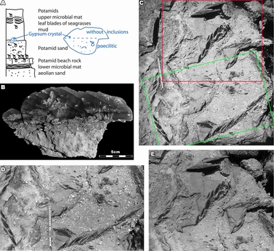
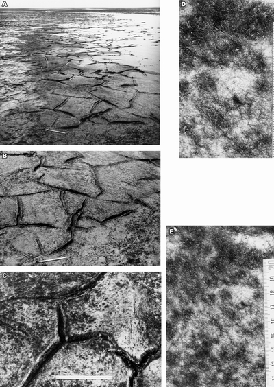
Figure
9: [by
courtesy of Jean-Claude Plaziat, Mussafah, February 1987]:
A) a section near the eastern end of the Mussafah channel displaying typical
facies including Potamid sands and beachrock, as well as the lower and the upper
microbial mats; B) detail of a syntaxial gypsum crystal, with inclusions
(poecilitic) and without; C-E) large gypsum crystals at the boundary between the
mud and the bioclastic sand. D corresponds to the green frame of C, and E to the
red frame. |
|
|
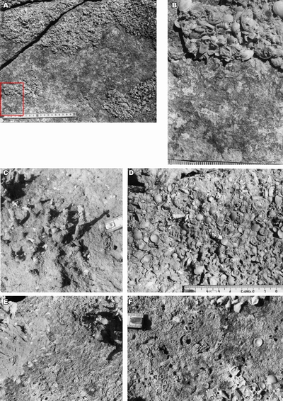
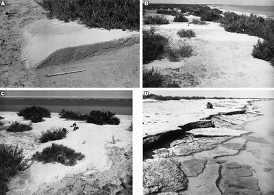
Figure
10: [by
courtesy of Jean-Claude Plaziat, Mussafah, February 1987]:
A-F) top of the Potamid beach-rock. B corresponds to the red frame of A. Erosion
of the Potamid shells (A-B, F) documents an early lithification followed by
mechanical abrasion. By contrast cementation of the more diverse assemblage of
shells found above the erosional surface (A-B, D) is probably not an" early
diagenetic event", i.e.,
lithification took place within the sedimentary pile; C) gypsiferous open
burrows in the Potamid sand above the Potamid beach rock; E) gypsiferous open
burrows (as in C) and surficial erosion of the early lithified Potamid beach
rock. |
|
|
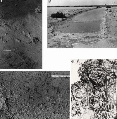
Figure
11: [by
courtesy of Jean-Claude Plaziat, Mussafah, February 1987]:
A)
microbial mats infilling on bottom of a residual pond in a former tidal
channel; B) healed desiccation cracks in the living microbial mat; C-D)
smooth
to felted surficial appearance of the microbial mat. |
|
|
Figure
12: [by
courtesy of Jean-Claude Plaziat, Mussafah, February 1987]:
A) The upper Potamid beach-rock at the edge of Mussafah channel near
7.2 km mark; B-C) modern sand blankets created by sediment transport from the
channel to its edges (washover fans) during storm events. There, plants bearing
yellow flowers (cf. orobanche /
broom-rape) are parasites of Salicornia
(Arthrocnemum spp.), a well-known
halophyte plant. |
|
|
Figure
13: [by
courtesy of Jean-Claude Plaziat, Mussafah, February 1987]: A) the upper part is a puddle of water
with living Potamids; the middle part is a zone with crab burrows; the
lower part is a zone with sand pellets made by "sand bubbler crabs", Scopimera
spp.; B) a small channel with Potamids on the side of Mussafah channel. At low
tide, it is disconnected from the main channel; C) detail of the zone with
living Potamids; D) a layer made of drift seagrass leaves found in the mud below
the upper microbial mat (Fig. 9.A |
|
|
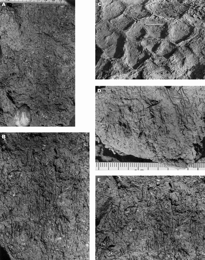
Figure 14: [by courtesy of Jean-Claude Plaziat, Mussafah, February 1987]: A-B & D-E) the muddy seagrass meadow facies with roots and a few rhizomes. In A, the pelecypod Anodontia edentula (Linnaeus, 1758); C) polygonal pattern after ? desiccation cracks of the upper microbial mat. |
Plate 1: Acetabularia Figs.
1-2: Calcified cap of an Acetabularia
sp. viewed from above. The scars of the fertile ampulae are visible on these
caps; |
|
|
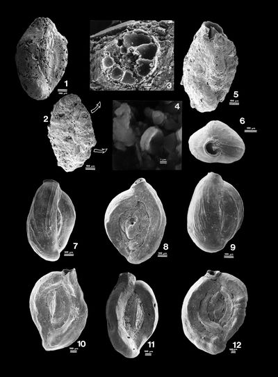
Plate 2: Spirorbis Fig. 1: Axial section of a Spirorbis
tube. Sample ABA 172, 6 km - G; |
|
|
Plate 3: Spirorbis and Diatoms Fig. 1: Encrusting basal surface of a Spirorbis tube
molding its non-fossilized support, a large piece either of seaweed or of
seagrass;
|
|
|
Plate 4: Spirorbis and Rhodophyta (Photos Hermes Brito, UNESPEtro) Fig. 1: Encrusting basal surface of a Spirorbis tube
molding encrusting Rhodophyta; [All scales represent 100 μm] |
|
|
Plate 5: Ostracods and small benthic Foraminifers Figs. 1-2: Gibboborchella sp. 1) left
valve; 2) dorsal view. |
|
|
Plate 6: Foraminifers Fig. 1: Elphidium sp., equatorial
section. Sample ABA 171, 4.2 km - G; |
|
|
Plate 7: Foraminifers: Miliolidae Fig. 1: Encrusted and bored test of a Quinqueloculina
sp., morphological type B of Murray, 1966; |
|
|
Plate 8: Foraminifers and faecal pellets Fig. 1: Sorites orbiculus (Forskal,
1775); |
|
|
Plate 9: Extraclasts Fig. 1: To the left, the subaxial section of an agglutinated Textulariid test
represents the main part of an extraclast found in the basal holocene Potamid beach-rock; to the right, the honey-colored section of
foraminifer is ascribed to a Peneroplis
sp. Sample ABA 167, 1.6 km - F; |
|
|
Plate 10: Extraclasts Fig. 1: This extraclast, i.e., a
lithoclast found in the Pleistocene sands, is made of calcitic ooids mostly
bonded by clotted micrite. Sample ABA 104, 14 D - V; |
|
|
Plate 11: Allochems Fig. 1: Gastropod shell in the basal Potamid
beach-rock. Fibrous cement has grown on the inner side of the shell.
Structureless grains, i.e.,
peloids, and grains with a fuzzy zoning, possible micritic ooids, are also found
in the former body cavity. Sample ABA 145, 0,6 km - D; |
|
|
Plate 12: Coccoids in a microbial mat Figs. 1-3: Scattered or aggregated calcified coccoid structures in the lower microbial mat. Sample ABA 165, 0 km - F. |
|
|
Plate 13: Coccoids in a microbial mat Fig. 1: Coccoids in the lower microbial mat. Scattered or aggregated calcified
coccoid structures, in association with filamentous structures (arrows), are
more or less easily discernible. Sample ABA 165, 0 km - F; |
|
|
Plate 14: Miscellanea Fig. 1:
A calcitic structure, probably a red alga, possibly Bostrychia
arbuscula Harvey, 1855, found in a mostly dolomitic intraclast
of the lower microbial mat. Sample ABA 129, 2 km - A; |
|
|
Plate 15: Diagenesis Fig. 1: "Rounded grain" with scattered calcite crystals (cement). Sample ABA 134,
4.2 km - B; |
|
|
Plate 16: Gypsum Fig. 1: Lower microbial mat sandwiched between the Pleistocene aeolian sands below
and the Holocene lithified Potamid sands above. 0.8 km; |
|